First, we'll try to understand what a Turing machine is informally. Remember that we started out with the finite automaton, considered the simplest model of computation. This is just some finite set of states, or memory, and some transitions. We can do a lot of useful things with FAs but there are many languages that FAs aren't powerful enough to recognize, such as $a^n b^n$. However, we can enhance the power of the machine by adding a stack. This gives us the ability to recognize a larger class of languages.
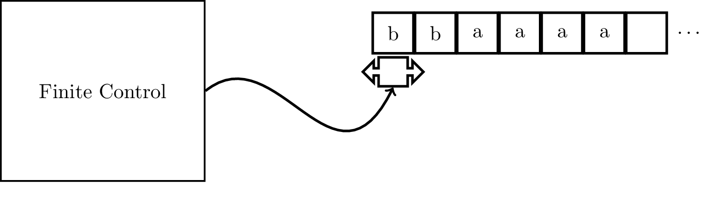
We can think of a Turing machine in the same way. A Turing machine is just a finite automaton with the two main restrictions we placed on it now lifted. That is, the tape that we placed our input on before which was read-only can now be written, and our tape is infinitely long. Furthermore, we can move however we like on the tape, unlike the pushdown stack.
A Turing machine is a 7-tuple $M = (Q,\Sigma,\Gamma,\delta,q_i,q_A,q_R)$, where
In our model, we have a one-sided infinitely long tape, with the machine starting its computation with the input on the tape beginning at the left end of the tape. The input string is followed by infinitely many blank symbols $\Box$ at the right.
We should note that this view of the Turing machine is kind of ahistorical. The Turing machine was introduced by Turing in 1936, while the finite automaton model was introduced by Kleene in the 50's. It's obvious now that the two are related and it's very helpful to relate the two models in this way, but Turing definitely didn't think of the machines he defined like this. In fact, near the end of Kleene's 1951 technical report, he devotes a paragraph or two discussing the possible similarities between his model and Turing's.
Instead, what Turing attempted to do was formalize how computers worked, by which we mean the 1930s conception of what a computer is. In other words, he tried to formalize how human computers might compute a problem. We can view the finite state system as a set of instructions we might give to a person, that tells them what to do when they read a particular symbol. We allow this person to read and write on some paper and we let them have as much paper as they want.
In the course of this computation, one of three outcomes will occur.
For a Turing machine $M$ and an input word $w$, if the computation of $M$ on $w$ enters the accepting state, then we say that $M$ accepts $w$. Likewise, if the computation of $M$ on $w$ enters the rejecting state, then we say $M$ rejects $w$.
We call the set of strings that are accepted by $M$ the language of $M$, denoted $L(M)$.
A Turing machine $M$ recognizes a language $L$ if every word in $L$ is accepted by $M$ and for every input not in $L$, $M$ either rejects the word or does not halt. A language $L$ is recognizable if some Turing machine recognizes it.
A Turing machine $M$ decides a language $L$ if every word in $L$ is accepted by $M$ and every input not in $L$ is rejected by $M$. A language $L$ is decidable if some Turing machine decides it.
When we talk about Turing machines, it's helpful to talk about the state that they're in. For Turing machines, the "state" of the machine is really a combination of three settings, which together are referred to as a configuration. A configuration specifies the particular state of a Turing machine during computation. More specifically, a configuration is defined by the state, the tape head position, and the contents of the tape.
For a state $q$ and two strings $u, v \in \Gamma^*$, we write $uqv$ for the configuration where the current state is $q$, the current tape contents is $uv$ and the tape head is located on the first symbol of $v$.
First, we'll define a Turing machine for the language $L = \{a^n b^n c^n \mid n \geq 0\}$. The operation of the machine can be described as follows:
The machine, when formally defined looks like this:
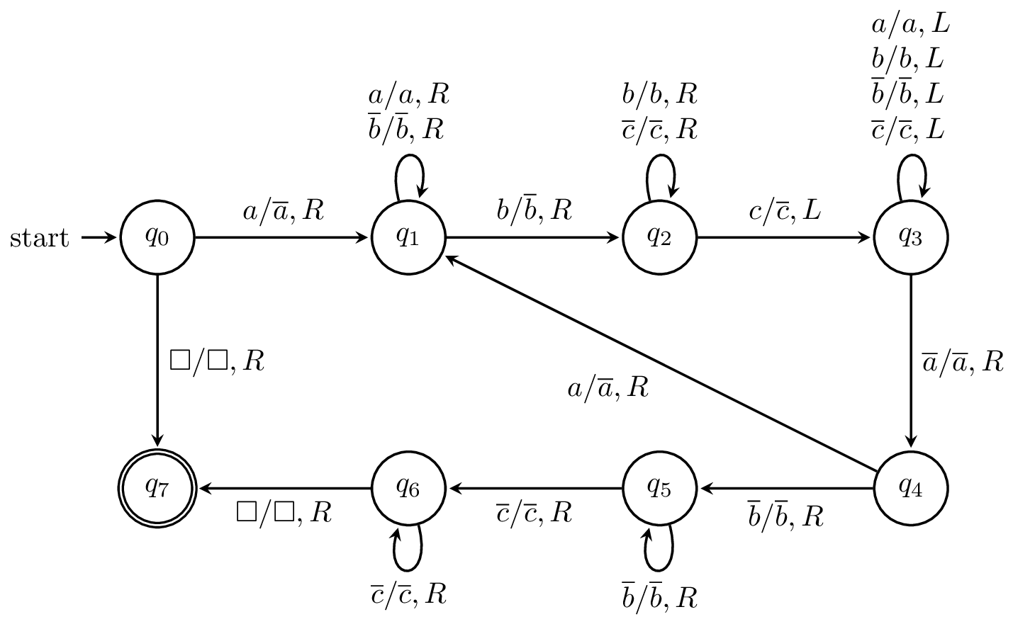
This will be the only time we see a Turing machine completely defined.
Next, we have the language of palindromes $L_{copy} = \{ x \# x \mid x \in \Sigma^* \}$. In other words, this is the language where we have two copies of the same word divided by $\#$. We've seen already that this language is not context-free. We can describe the machine as follows: