We have moved from talking about the probability of events to thinking about the probability of a property of events, in the form of random variables. Now, if we know these probabilities, we can ask the question of what kinds of values we might expect more often.
Let $(\Omega,\Pr)$ be a probability space and let $X$ be a random variable. The expected value of $X$ is \[E(X) = \sum_{\omega \in \Omega} X(\omega) \Pr(\omega).\]
Roughly speaking, the expectation of a random variable is the (weighted) average value for the random variable.
Consider a fair 6-sided die and let $X$ be the random variable for the number that was rolled. We have \[E(X) = 1 \cdot \frac 1 6 + 2 \cdot \frac 1 6 + 3 \cdot \frac 1 6 + 4 \cdot \frac 1 6 + 5 \cdot \frac 1 6 + 6 \cdot \frac 1 6 = \frac{21}{6} = 3.5.\] Now, consider a biased 6-sided die with \[\Pr(\omega) = \begin{cases} \frac 3 4 & \text{if $\omega = 1$,} \\ \frac{1}{20} & \text{otherwise}. \end{cases}\] Let $Y$ be the random variable for the number that was rolled with our biased die. Then we get \[E(Y) = 1 \cdot \frac 3 4 + 2 \cdot \frac{1}{20} + 3 \cdot \frac{1}{20} + 4 \cdot \frac{1}{20} + 5 \cdot \frac{1}{20} + 6 \cdot \frac{1}{20} = \frac 3 4 + \frac{20}{20} = 1.75.\] This indicates to us that the biased die will give us a 1 more often and therefore the average value that we should expect from a roll is much closer to 1.
It's important to note that what this tells us is not that we should expect a fair die roll to be 3.5 or 1.75 when we roll it, because obviously that will never happen. Rather, what expectation tells us is that, over time, the more we roll the die, the closer the value of the average roll will be to 3.5 or 1.75.
Recall that the motivation for defining random variables was so we could get away from considering the probabilities of elementary events. The definition of expectation is not very helpful in this regard. Luckily, it is not too difficult to reformulate expectation in terms of the values that the random variable takes on.
Let $\Pr(X = r) = \Pr(\{\omega \mid X(\omega) = r\})$ and let $\{r_1, \dots, r_k\} = \operatorname{range}(X)$. Then \[E(X) = \sum_{i=1}^k r_i \cdot \Pr(X = r_i).\]
Recall that the range of a function $X$ is all of the possible values that $X(\omega)$ can take over every $\omega \in \Omega$. Then we have \begin{align*} \sum_{i=1}^k r_i \cdot \Pr(X = r_i) &= \sum_{i=1}^k r_i \cdot \Pr(\{\omega \in \Omega \mid X(\omega) = r_i\}) \\ &= \sum_{i=1}^k r_i \cdot \sum_{\omega \in \Omega, X(\omega) = r_i} \Pr(\omega) \\ &= \sum_{i=1}^k \sum_{\omega \in \Omega, X(\omega) = r_i} X(\omega) \Pr(\omega) \\ &= \sum_{\omega \in \Omega} X(\omega) \Pr(\omega) \\ &= E(X) \end{align*}
Sometimes, we will need to deal with more than one random variable. For instance, suppose we want to consider the expected value of a roll of three dice. We would like to be able to use the expected value for a single die roll, which we already worked out above. The following result gives us a way to do this.
Let $(\Omega, \Pr)$ be a probability space, $c_1, c_2, \dots, c_n$ be real numbers, and $X_1, X_2, \dots, X_n$ be random variables over $\Omega$. Then \[E\left( \sum_{i=1}^n c_i X_i \right) = \sum_{i=1}^n c_i E(X_i).\]
Suppose we have three of our biased dice from the previous example, each with $\Pr(1) = \frac 3 4$ and probability $\frac{1}{20}$ for the other outcomes. What is the expected value of a roll of these three dice? Without the linearity property, we would need to consider the expected value for every 3-tuple of rolls $(\omega_1, \omega_2, \omega_3)$. However, we can apply the previous theorem to get a more direct answer. Let $X_1, X_2, X_3$ be random variables for the roll of each die. Then we have \[E(X_1 + X_2 + X_3) = E(X_1) + E(X_2) + E(X_3) = 1.75 + 1.75 + 1.75 = 5.25.\]
Something you may have noticed is that from our previous discussions, in a roll of three dice, the roll of each die is independent from the others. Recall from last week's problem set the definition of independence for random variables:
We say the random variables $X$ and $Y$ are independent if for all $r,s \in \mathbb R$, $\Pr(X = r \wedge Y = s) = \Pr(X = r) \cdot \Pr(Y = s)$.
It is important to note that although we have a very similar notion of independence for random variables, none of our results so far have involved independence. That is, the linearity of expectation does not depend on the independence of the random variables involved. In fact, one can show that every random variable can be rewritten as a linear combination of indicator variables.
Consider a random permutation $\pi$ of $\{1, 2, \dots, n\}$. A pair $(i,j)$ is an inversion in $\pi$ if $i \lt j$ and $j$ precedes, or appears before, $i$ in $\pi$. What is the expected number of inversions in $\pi$?
Let $I_{i,j}$ be the random variable with $I_{i,j} = 1$ if $i \lt j$ and $(i,j)$ is an inversion and $I_{i,j} = 0$ otherwise. Let $X$ be the random variable for the number of inversions in a permutation. Then \[X = \sum_{1 \leq i \lt j \leq n} I_{i,j}.\] Then we have \[E(X) = \sum_{1 \leq i \lt j \leq n} E(I_{i,j}).\] So, what is $E(I_{i,j})$? If we consider all permutations, then half of them will have $i \lt j$ and the other half will have $j \lt i$. This gives us $E(I_{i,j}) = \frac 1 2$. Then, we count the number of pairs $(i,j)$ with $i \lt j$ to get the number of terms in our summation. There are $\binom n 2$ such pairs, since we pick any pair of numbers and there's only one possible order we care about. This gives us \[E(X) = \sum_{1 \leq i \lt j \leq n} E(I_{i,j}) = \binom n 2 \frac 1 2 = \frac{n(n-1)}2 \frac 1 2 = \frac{n(n-1)}4.\]
This leads us to a nice average-case analysis of bubble sort. As you may recall, bubble sort involves going through an array and checking if each pair of adjacent elements is in the right order and swaps them if they're not. The worst-case analysis comes when we have an array that's totally in reverse, and we're forced to make $n$ passes through the array making $O(n)$ swaps, giving us a running time of $O(n^2)$.
Of course, a common criticism of worst-case analysis is that it's possible that typical cases aren't that bad. So for this case, we can ask ourselves, if we have a random array, how many swaps would we expect to make? This happens to be asking how many pairs of numbers we should expect to be out of order in a random permutation, which we've just figured out is $\frac{n(n-1)}4$. And so it turns out, in the average case, we're still looking at a running time of $O(n^2)$.
Up until now, we've been considering a sequence of trials of some fixed length. But sometimes, we may want to perform a sequence of trials until we get a success. This means that we are working with an infinite sample space and we can be potentially waiting for a long time. However, we can show that we can put an estimate on how long we should expect to wait.
Let $X$ be a Bernoulli trial with probability of success $p$. The expected number of trials before the first success is $\frac 1 p$.
First, we note that we are interested in events where there is exactly one success, which is the final trial. After we see a success, we can stop performing trials. So suppose we perform $k$ trials and the last one is the success. Let $Y$ be the random variable equal to the number of trials of $X$ that are performed, with a final success. Then we have \[\Pr(Y = j) = (1-p)^{j-1} p\] since we needed to perform $j-1$ failures before getting a success. Then the expected number of trials is \[E(Y) = \sum_{j=0}^\infty j \cdot \Pr(Y=j) = \sum_{j=1}^\infty j(1-p)^{j-1}p = p \sum_{j=1}^\infty j (1-p)^{j-1}.\] Note here that we take out the term for $Y=0$, since that term is 0 and doesn't contribute to the sum. Now, we apply the following very useful identity: \[\sum_{k=1}^\infty k x^{k-1} = \frac 1 {(1-x)^2}.\] Setting $k = j$ and $x = 1-p$ gives us \[\sum_{j=1}^\infty j (1-p)^{j-1} = \frac 1 {(1-(1-p))^2} = \frac 1{p^2}.\] Then we have \[p \sum_{j=1}^\infty j (1-p)^{j-1} = p \cdot \frac 1 {p^2} = \frac 1 p.\]
The 3-satisfiability problem is one of the most famous "difficult" problem in computer science. The problem asks, when given a propositional formula in conjunctive normal form where each clause has three literals, whether there is an assignment of variables that makes the formula evaluate to true. Here, a clause is three variables or their negations joined together by $\vee$. Each clause is joined by $\wedge$. For example, \[(x_1 \vee \neg x_2 \vee x_4) \wedge (x_2 \vee x_3 \vee \neg x_4) \wedge (\neg x_1 \vee \neg x_3 \vee x_5).\]
One (also difficult) variant of this problem asks for an assignment that makes as many clauses true as possible. This is difficult, because if there are $n$ variables, we have to look through as many as $2^n$ different assignments to see which one gives us the maximum number of satisfied clauses.
However, what if we just randomly guessed an assignment? Suppose we flip a coin independently for each variable $x_i$, setting it to True with probability $\frac 1 2$. How many clauses should we expect to satisfy? Our claim is the following.
Let $\varphi$ be a formula in 3-CNF with $k$ clauses. we should expect that $\frac 7 8$ of them will be satisfied—perhaps surprisingly large.
Let's name our clauses $C_1, \dots, C_k$. Define the random variable $Z_j$ by \[Z_j = \begin{cases} 1 & \text{if clause $C_j$ is satisfied}, \\ 0 & \text{otherwise}. \end{cases}\] Then we define the random variable $Z$ to be the number of clauses that have been satisfied. That is, $Z = Z_1 + \cdots + Z_k$. We can then compute $E(Z)$ by figuring out $E(Z_j)$ for a single clause. But what is $E(Z_j)$?
Let's consider the possible assignments we can make to a clause $(x \vee y \vee z)$. There are three literals and each one can take on two values, so there are as many as 8 possible assignments. However, we observe that the clause is satisfied as long as one literal evaluates to True. In other words, in order for the clause not to be satisfied, all three literals must evaluate to False. There is only one possible assignment that does this, with probability $\frac 1 8$, which means that the probability that our clause is satisfied is $1 - \frac 1 8 = \frac 7 8$.
So $E(Z_j) = \frac 7 8$ for all $j$. This gives us \[E(Z) = \sum_{j=1}^k E(Z_j) = \sum_{j=1}^k \frac 7 8 = \frac 7 8 k.\]
This is a nice result, which tells us a bit more than what we came here for. This result says that if we have a random assignment, we can expect to satisfy $\frac 7 8$ of the clauses. Now, notice that we may not be guaranteed this number—we may end up satisfying fewer. However, the implication is that we could also end up satisfying more, which gives us an interesting result: there has to exist an assignment of variables that satisfies at least $\frac 7 8$ of the clauses.
This is another result that uses the probabilistic method—we showed that there is a nonzero probability that such an assignment exists. However, we don't have any way of finding it easily, which doesn't really help us solve the problem. Or does it?
Suppose we extend our previous strategy. Instead of just randomly assigning variables and taking the result, what if we kept on coming up with random assignments until we get an assignment that satisfies at least $\frac 7 8$ of the clauses? Luckily, we proved a very useful theorem about this. But first, we have to find the probability that an assignment will satisfy at least $\frac 7 8$ of the clauses.
Let $\varphi$ be a formula in 3-CNF with $k$ clauses. The probability that a random assignment satisfies at least $\frac 7 8 k$ clauses is at least $\frac 1 {8k}$.
Let $p_j$ denote the probability that exactly $j$ clauses are satisfied by a random assignment. We want to compute the probability $p = \sum\limits_{j \geq \frac 7 8 k} p_j$ that at least $\frac 7 8 k$ clauses are satisfied. By definition, we have \[E(Z) = \frac 7 8 k = \sum_{j=0}^\infty j p_j.\] We split this sum into two: \[\sum_{j=0}^\infty j p_j = \sum_{j \lt \frac 7 8 k} j p_j + \sum_{j \geq \frac 7 8 k} j p_j.\] We note in the first sum that $j$ ranges from 0 to just under $\frac 7 8 k$, which gives us \[\sum_{j \lt \frac 7 8 k} j p_j \leq \left(\frac 7 8 k - \frac 1 8\right) \sum_{j \lt \frac 7 8 k} p_j.\] Similarly, the second sum has $j$ ranging from $\frac 7 8 k$ to $k$, the total number of clauses. This gives us \[\sum_{j \geq \frac 7 8 k} j p_j \leq k \sum_{j \geq \frac 7 8 k} p_j.\] Together, we have \begin{align*} \sum_{j=0}^\infty j p_j &= \sum_{j \lt \frac 7 8 k} j p_j + \sum_{j \geq \frac 7 8 k} j p_j \\ &\leq \left(\frac 7 8 k - \frac 1 8\right) \sum_{j \lt \frac 7 8 k} p_j + k \sum_{j \geq \frac 7 8 k} p_j \\ &= \left(\frac 7 8 k - \frac 1 8 \right) \cdot (1-p) + k p \\ &\leq \left(\frac 7 8 k - \frac 1 8 \right) + k p \end{align*} To summarize, we have \[\frac 7 8 k \leq \left(\frac 7 8 k - \frac 1 8 \right) + k p.\] We rearrange this to solve for $p$: \begin{align*} \left(\frac 7 8 k - \frac 1 8 \right) + k p &\geq \frac 7 8 k \\ k p &\geq \frac 7 8 k - \left(\frac 7 8 k - \frac 1 8 \right) \\ k p &\geq \frac 1 8 \\ p &\geq \frac 1 {8k} \end{align*}
Using this result, we can conclude that we expect the number of assignments we need to try (i.e. the number of trials before a success) is $8k$, which is linear in the size of a 3-CNF formula. This leads to a straightforward Monte Carlo algorithm. Monte Carlo algorithms are algorithms that have some chance of producing an "incorrect" answer (in this case, an assignment that satisfies fewer than $\frac 7 8$ths of the clauses). The key insight that makes Monte Carlo algorithms work is the waiting time bound: we can simply retry our algorithm until we have a good enough answer, and we can prove a bound on how many times we expect to re-run it.
A question we can ask about expectations and random variables is what the probability that a random variable takes on a value that is far from the expected value? Intuitively, this shouldn't happen very often. The following result will give us a rough bound on the probability that a random variable takes on a value of at least some constant $a$.
If $X$ is nonnegative, then $\forall a \gt 0$, \[\Pr(X \geq a) \leq \frac{E(X)}{a}.\]
\begin{align*} E(X) &= \sum_{\omega \in \Omega} X(\omega) \Pr(\omega) \\ &\geq \sum_{\omega \in \Omega, X(\omega) \geq a} X(\omega) \Pr(\omega) \\ &\geq \sum_{\omega \in \Omega, X(\omega) \geq a} a \cdot \Pr(\omega) \\ &= a \cdot \sum_{\omega \in \Omega, X(\omega) \geq a} \Pr(\omega) \\ &= a \cdot \Pr(X \geq a). \end{align*}
This gives us $\Pr(X \geq a) \leq \frac{E(X)}{a}$.
Markov's inequality is named for Andrey Markov, a Russian mathematician from the turn of the 20th century who is the same Markov responsible for things like Markov chains. Interestingly enough, this inequality appeared earlier in work by Pafnuty Chebyshev, who was Markov's doctoral advisor.
Intuitively, this result tells us that the larger, and therefore further away from the expected value, that the result of a random variable takes on, the less likely it is to do so.
Let $X$ be the random variable for the number of heads when a fair coin is tossed $n$ times. Recall that this is just the number of successful outcomes for $n$ independent Bernoulli trials with $p = \frac 1 2$. One can calculate that $E(X) = \frac n 2$.
Let's consider an estimate by Markov's inequality. If we set $a = 60$ and $n = 100$, we get an upper bound on the probability that we get more than 60 heads in 100 coin flips. This gives us \[Pr(X \geq 60) \leq \frac{\frac{100}2}{60} = \frac 5 6.\] So Markov's inequality tells us the probability that we get more than 60 heads is at most just over 80%, which seems kind of high. So you can guess that this inequality, though simple, does not give an incredibly great estimate.
Still, we can derive a useful, if obvious fact from this: a random variable $X$ must take on a value at least as large as $E(X)$ some of the time.
Let $X$ be a random variable. Then $\Pr(X \geq E(X)) \gt 0$.
Suppose for contradiction that $\Pr(X \lt E(X)) = 1$. Then we can define a random variable $Y = E(X) - X$, which is always positive. By linearity of expectation, we have $E(Y) = E(X) - E(X) = 0$. But since $Y$ is nonnegative, we can apply Markov's inequality. Therefore, we have for all $a \gt 0$, \[\Pr(Y \geq a) \leq \frac{E(Y)} a = \frac 0 a = 0.\] But since this is true for any $a \gt 0$, this says that $\Pr(Y \gt 0) \leq 0$. Therefore, $\Pr(Y = 0) = 1$, which contradicts our assumption that $Y$ is always strictly positive.
This is the fact that we took advantage of when trying to find an assignment of variables in MAX-3SAT: since the expected number of satisfying clauses for a random assignment of variables is $\frac 7 8 k$, there has to be some assignment that exists that satisfies at least that many clauses.
However, beyond just the issue of providing fairly rough bounds, one problem with Markov's inequality is that it really only works in one direction. Intuitively, we should be able to bound the probability that a random variable takes on values far away from the expectation in both directions. In other words, we would like and expect that the outcomes of a random variable $X$ should be concentrated around $E(X)$ with high probability.
This leads us to the following notions.
Let $X$ be a random variable on the probability space $(\Omega,\Pr)$. The variance of $X$ is \[V(X) = \sum_{\omega \in \Omega} (X(\omega) - E(X))^2 \cdot \Pr(\omega).\] The standard deviation of $X$ is $\sigma(X) = \sqrt{V(X)}$. Because of this, variance is sometimes denoted by $\sigma^2(X)$.
Again, the definition of variance is in terms of the probabilty of events from $\Omega$, which is not ideal. Luckily, we can reformulate variance in terms of the expectation of $X$ only.
If $X$ is a random variable, then $V(X) = E(X^2) - E(X)^2$.
\begin{align*} V(X) &= \sum_{\omega \in \Omega} (X(\omega) - E(X))^2 \cdot \Pr(\omega) \\ &= \sum_{\omega \in \Omega} (X(\omega)^2 - 2X(\omega)E(X) + E(X)^2) \cdot \Pr(\omega) \\ &= \sum_{\omega \in \Omega} X(\omega)^2 \cdot \Pr(\omega) - 2 E(X) \sum_{\omega \in \Omega} X(\omega) \cdot \Pr(\omega) + E(X)^2 \sum_{\omega \in \Omega} \Pr(\omega) \\ &= E(X^2) - 2E(X)^2 + E(X)^2 \\ &= E(X^2) - E(X)^2 \end{align*}
$V(X) = E((X - E(X))^2)$.
Recall the roll of a fair 6-sided die and that $E(X) = 3.5$. To compute the variance, we need $E(X^2)$. For $i = 1, 2, \dots, 6$, $X^2 = i^2$ with probability $\frac 1 6$. Then \[E(X^2) = \sum_{i=1}^6 \frac{i^2}{6} = \frac{91}6.\] Then we can calculate $V(X)$ by \[V(X) = E(X^2) - E(X)^2 = \frac{91}{6} - \left( \frac 7 2 \right)^2 = \frac{35}{12} \approx 2.92.\] From this, we can also get the standard deviation, $\sqrt{V(X)} \approx 1.71$.
Now, what if we wanted to consider the roll of more than one die? Recall that the result of mulitple die rolls is independent and so their corresponding random variables are independent. We can make use of this property via Bienaymé's formula. Irénée-Jules Bienaymé was a French mathematician at around the same time as Markov and Chebyshev and was friends and collaborators with Chebyshev.
If $X$ and $Y$ are independent random variables, then $V(X+Y) = V(X) + V(Y)$.
Recall that the variance of a single die roll is $V(X) = \frac{35}{12}$. Then the variance of two die rolls is $V(X) + V(X) = \frac{35}{6} \approx 5.833$ and the standard deviation is about $2.42$.
Consider a series of $n$ independent Bernoulli trials with probability of success $p$. What is the variance of the number of successes?
As in our usual setup of series of independent Bernoulli trials, we define the random variable $X_i$ to be 1 if $a_i$ is a success and 0 otherwise and $X = X_1 + \cdots + X_n$, he number of successes in the $n$ trials. However, unlike expectation, we do need to rely on the fact that the $X_i$'s are independent in order to apply Bienaymé's formula to get $V(X) = V(X_1) + \cdots + V(X_n)$.
Luckily, this means that, as with expectation, we just need to compute the variance of a single Bernoulli trial. If $X_i$ is our random variable for the Bernoulli, trial, we have that $X_i$ takes on a value of either 0 or 1. Therefore, we have $X_i^2 = X_i$ and $E(X_i) = 1 \cdot p + 0 \cdot (1-p) = p$. Then \[V(X_i) = E(X_i^2) - E(X_i)^2 = p - p^2 = p \cdot (1-p).\] This gives us, we have $V(X) = np(1-p)$.
The following result, due to Chebyshev, will improve on Markov's inequality to give us a better bound on how much a random variable differs from its expected value, but using the variance of the random variable.
Let $X$ be a random variable. For all $a \gt 0$, \[\Pr(|X - E(X)| \geq a) \leq \frac{V(X)}{a^2}.\]
Let $Y = (X - E(X))^2$ be a random variable. Then $E(Y) = V(X)$ by definition. We can apply Markov's inequality, since $Y$ is non-negative, to get \[\Pr(Y \geq a^2) \leq \frac{E(Y)}{a^2}.\] Since $Y = (X-E(X))^2$, consider $(X-E(X))^2 \geq a^2$. We have $(X-E(X))^2 \geq a^2$ if and only if $|X - E(X)| \geq a$. Then, together with $E(Y) = V(X)$, we substitute into the above to get \[\Pr(|X-E(X)| \geq a) \leq \frac{V(X)}{a^2}.\]
Let's revisit the example at the start of this section: what is the probability that we get more than 60 heads on 100 flips of a fair coin? Recall that if $X$ is the random variable for the number of heads when a fair coin is tossed $n$ times, then $E(X) = \frac n 2$. From the preceding example, we also have that $V(X) = \frac n 4$ (since $p = (1-p) = \frac 1 2$).
Now, let's apply Chebyshev's inequality. First, we can use $a = \sqrt n$ to get \[\Pr\left( \left|X - \frac n 2 \right| \geq \sqrt n \right) \leq \frac{V(X)}{\sqrt n^2} = \frac n 4 \cdot \frac 1 n = \frac 1 4.\]
What this says is there is at most a $\frac 1 4$ probability that the number of heads that we get differs from the expected number ($\frac 1 2)$ by more than $\sqrt n$. So, if we make 100 rolls, then we have \[\Pr(|X - 50| \geq 10) \leq \frac 1 4.\] In other words, the probability that we get more than 60 heads or less than 40 heads is at most $\frac 1 4$, which is already significantly better than our estimate from Markov's inequality (based on this information, we can actually take one more step to improve the estimate even further—how?).
You may be familiar with graphs as either graphical charts of data or from calculus in the form of visualizing functions in some 2D or 3D space. Neither of these are the graphs that are discussed in graph theory.
We've actually already seen two examples where graphs snuck in. The first is from our application of the pigeonhole principle to a problem about whether two people know each other or don't know each other at a party. The second is from the example of our ambitious travelling salesperson, who wants to visit as many cities as possible with the least cost.
Both of these examples model relationships between sets of objects. In the first case, we are modelling what's basically a social network. Our objects are people and the relationships are described as: two people are connected by either a "knows each other" relationship or a "doesn't know each other" relationship. In the second case, our objects are cities and their relationship is described not only by a connection, but by a weight or cost on that connection, representing the cost to travel between the two cities.
A graph $G = (V,E)$ is a pair with a non-empty set of vertices $V$ together with a set of edges $E$. An edge $e \in E$ is an unordered pair $(u,v)$ of vertices $u,v \in V$.
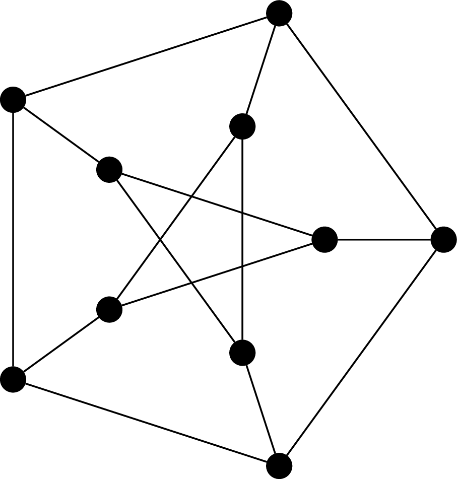
This graph is called the Petersen graph. The Petersen graph is a particularly interesting graph, not just because it looks neat, but because it happens to be a common counterexample for many results in graph theory.
Note that, since edges are unordered, we really should be writing them as $\{u,v\}$, but we don't.
One can define graphs more generally and then restrict consideration to our particular definition of graphs, which would usually be then called simple graphs. The more general definition of graphs allows for things like multiple edges between vertices or loops. Other enhancements may include asymmetric edges (which we call directed edges), equipping edges with weights, and even generalizing edges to hyperedges that relate more than two vertices. Instead, what we do is start with the most basic version of a graph, from which we can augment our definition with the more fancy features if necessary (it will not be necessary in this course).
Two vertices $u$ and $v$ of a graph $G$ are adjacent if they are joined by an edge $(u,v)$. We say the edge $(u,v)$ is incident to $u$ and $v$.
Two vertices $u$ and $v$ are neighbours if they are adjacent. The neighbourhood of a vertex $v$ is the set of neighbours of $v$ $$N(v) = \{u \in V \mid (u,v) \in E\}.$$ We can extend this definition to sets of vertices $A \subseteq V$ by $$N(A) = \bigcup_{v \in A} N(v).$$
The degree of a vertex $v$ in $G$, denoted $\deg(v)$, is the number of its neighbours. A graph $G$ is $k$-regular if every vertex in $G$ has degree $k$.
Observe that every vertex in the Petersen graph has degree 3, so the Petersen graph is 3-regular, or cubic.
The following results are some of the first graph theory results, proved by Leonhard Euler in 1736.
Let $G = (V,E)$ be an undirected graph. Then $$\sum_{v \in V} \deg(v) = 2 \cdot |E|.$$
Every edge $(u,v)$ is incident to exactly two vertices: $u$ and $v$. Therefore, each edge contributes 2 to the sum of the degrees of the vertices in the graph.
Now, let's look at some examples of some well-known graphs.
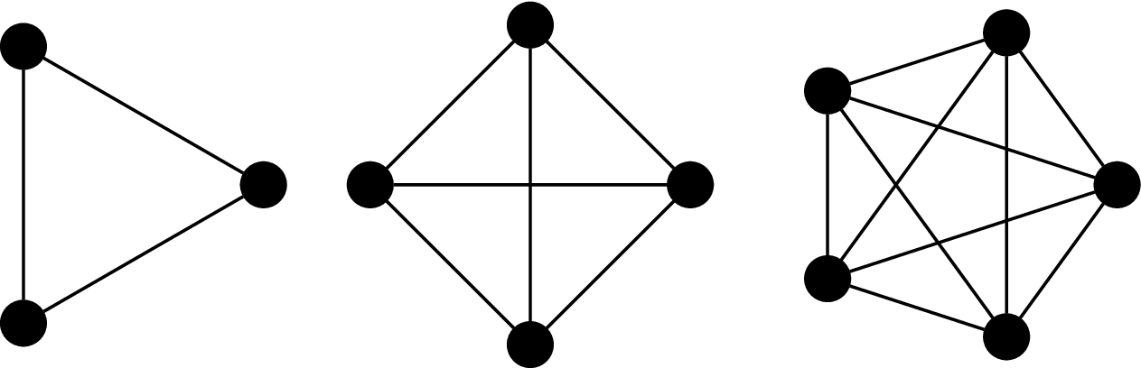
The complete graph on $n$ vertices is the graph $K_n = (V,E)$, where $|V| = n$ and
$$E = \{(u,v) \mid u,v \in V\}.$$
That is, every pair of vertices are neighbours.
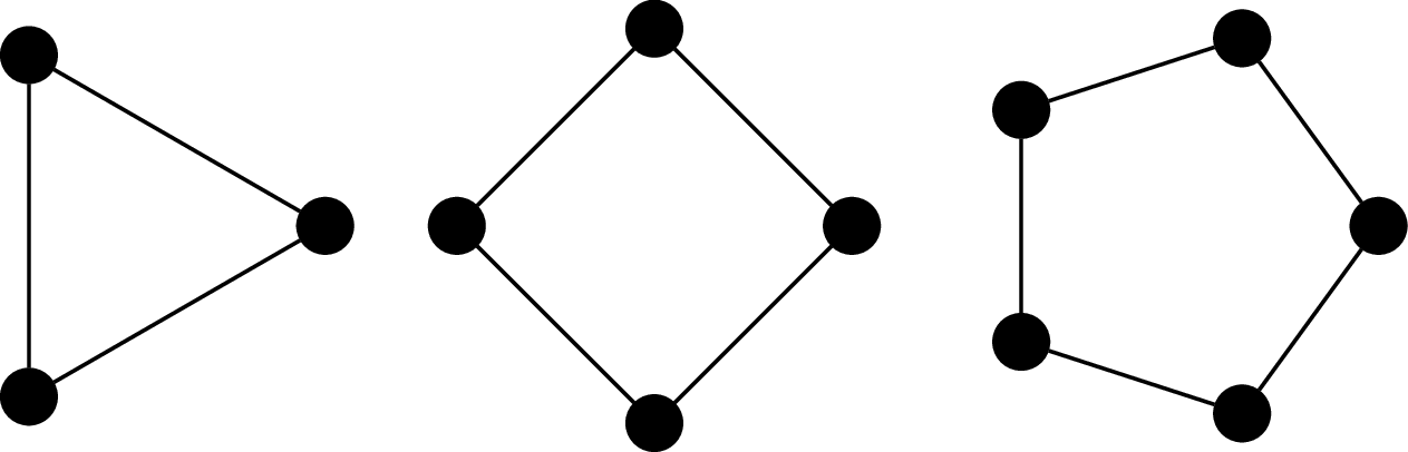
The cycle graph on $n$ vertices is the graph $C_n = (V,E)$ where $V = \{v_1, v_2, \dots, v_n\}$ and $E = \{(v_i,v_j) \mid j = i + 1 \bmod n\}$. It's named so because the most obvious way to draw the graph is with the vertices arranged in order, on a circle.
The $n$-(hyper)cube graph is the graph $Q_n = (V,E)$, where $V = \{0,1\}^n$ (i.e., binary strings of length $n$) and $(u,v)$ is an edge if, for $u = a_1 a_2 \cdots a_n$ and $v = b_1 b_2 \cdots b_n$, there exists an index $i, 1 \leq i \leq n$ such that $a_i \neq b_i$ and $a_j = b_j$ for all $j \neq i$. In other words, $u$ and $v$ differ in exactly one symbol.
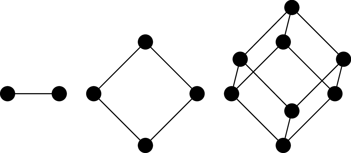
It's called a cube (or hypercube) because one of the ways to draw it is to arrange the vertices and edges so that they form the $n$th-dimensional cube.
Consider the following graphs.
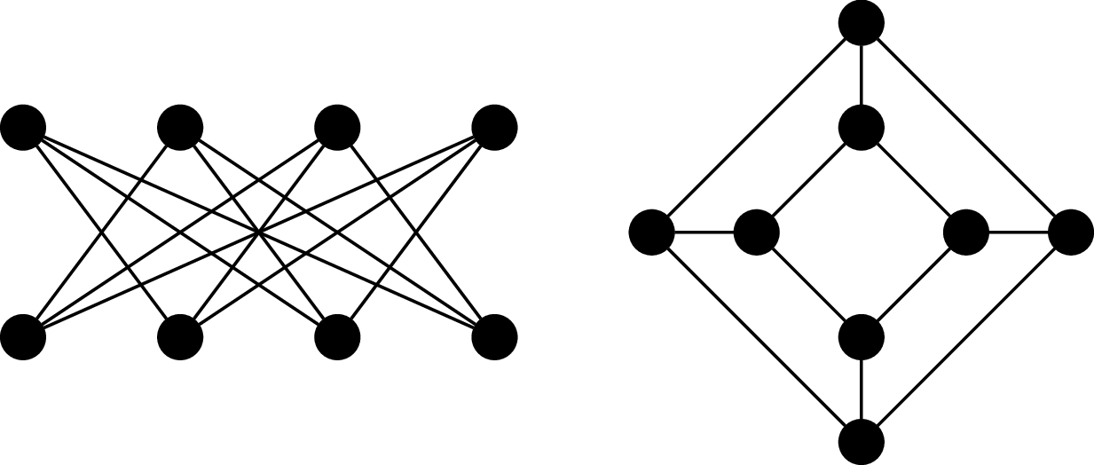
These two graphs happen to be the "same". Furthermore, it turns out that these are also basically the same graph as $Q_3$, or at least, we feel that it should be. This means we don't need to necessarily draw a $3$-cube like a cube (and we certainly wouldn't expect this for $n \gt 3$).
Although the visual representation of the graph is very convenient, it is sometimes misleading, because we're limited to 2D drawings. In fact, there is a vast area of research devoted to graph drawing and the mathematics of embedding graphs in two dimensions. The point of this is that two graphs may look very different, but turn out to be the same.
But even more fundamental than that, we intuitively understand that just because the graph isn't exactly the same (i.e., the vertices are named something differently) doesn't mean that we don't want to consider them equivalent. So how do we discuss whether two graphs are basically the same, just with different names or drawings?
An isomorphism between two graphs $G_1 = (V_1,E_1)$ and $G_2 = (V_2,E_2)$ is a bijection $f:V_1 \to V_2$ which preserves adjacency. That is, for all vertices $u,v \in V_1$, $u$ is adjacent to $v$ in $G$ if and only if $f(u)$ and $f(v)$ are adjacent in $G_2$. Two graphs $G_1$ and $G_2$ are isomorphic if there exists an isomorphism between them, denoted $G_1 \cong G_2$.
In other words, we consider two graphs to be the "same" or equivalent if we can map every vertex to the other graph such that the adjacency relationship is preserved. In practice, this amounts to a "renaming" of the vertices, which is what we typically mean when we say that two objects are isomorphic. Of course, this really means that the edges are preserved.
Consider the following graphs $G_1 = (V_1, E_1)$ and $G_2 = (V_2, E_2)$.
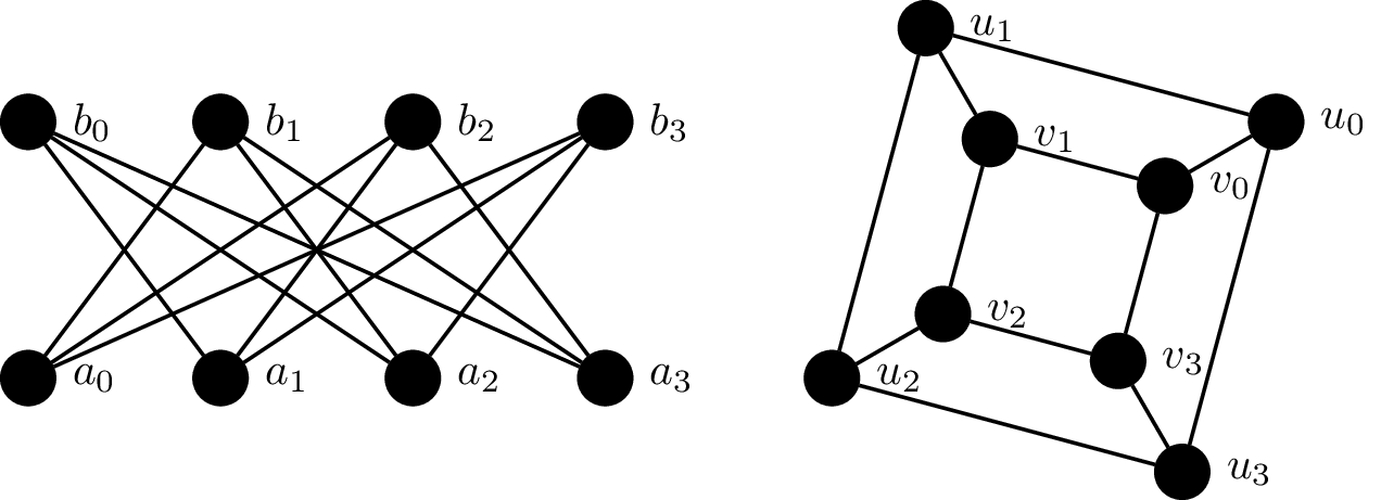
We will show that these two graphs are isomorphic by defining a bijective function $f:V_1 \to V_2$ which preserves adjacency: \begin{align*} f(a_0) &= u_0 & f(a_1) &= v_3 & f(a_2) &= u_2 & f(a_3) &= v_1 \\ f(b_0) &= v_2 & f(b_1) &= u_1 & f(b_2) &= v_0 & f(b_3) &= u_3 \\ \end{align*} This is a bijection, since every vertex in $V_1$ is paired with a vertex in $V_2$. We then verify that this bijection preserves adjacency by checking each edge under the bijection: \begin{align*} (f(a_0),f(b_1)) &= (u_0,u_1) & (f(a_0),f(b_2)) &= (u_0,v_0) & (f(a_0),f(b_3)) &= (u_0,u_3) \\ (f(a_1),f(b_0)) &= (v_3,v_2) & (f(a_1),f(b_2)) &= (v_3,v_0) & (f(a_1),f(b_3)) &= (v_3,u_3) \\ (f(a_2),f(b_0)) &= (u_2,v_2) & (f(a_2),f(b_1)) &= (u_2,u_1) & (f(a_2),f(b_3)) &= (u_2,u_3) \\ (f(a_3),f(b_0)) &= (v_1,v_2) & (f(a_3),f(b_1)) &= (v_1,u_1) & (f(a_3),f(b_2)) &= (v_1,v_0) \end{align*}
So an obvious and fundamental problem that arises from this definition is: Given two graphs $G_1$ and $G_2$, are they isomorphic? The obvious answer is that we just need to come up with an isomorphism or show that one doesn't exist. Unfortunately, there are $n!$ possible such mappings we would need to check.
There are a few ways we can rule out that graphs aren't the same, via properties that we call isomorphism invariants. There are properties of the graph that can't change via an isomorphism, like the number of vertices or edges in a graph.
A $k$-colouring of a graph is a function $c : V \to \{1,2,\dots,k\}$ such that if $(u,v) \in E$, then $c(u) \neq c(v)$. That is, adjacent vertices receive different colours. A graph is $k$-colourable if there exists a $k$-colouring for $G$.
We will use $k$-colourability as an invariant to show that two graphs are not isomorphic.
Consider the following two graphs, $G_1$ and $G_2$.
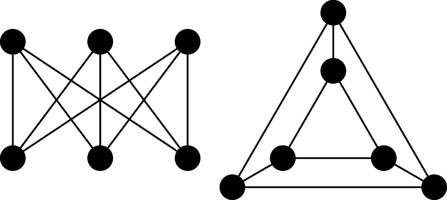
First, we observe that both graphs have 6 vertices and and 9 edges and both graphs are 3-regular. However, we will show that $G_1$ is 2-colourable and $G_2$ is not. To see that $G_1$ is 2-colourable, we observe that the vertices along the top row can be assigned the same colour because they are not adjacent to each other. Similarly, the vertices along the bottom can be assigned a second colour.
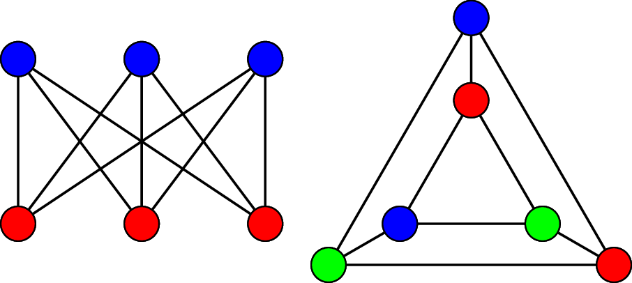
However, $G_2$ contains two triangles and by definition, the vertices belonging to the same triangle must be coloured with 3 different colours. Since $G_2$ is not 2-colourable, the adjacency relationship among the vertices is not preserved.