Rows and rank
Let's go back to our factorization $A = CR$ and recall that one interpretation of this product is that each column of $R$ describes how to combine columns of $C$ to construct a column of $A$.
Notice that each row of $R$ is associated with a column of $C$. We can "decompose" our product in a different way.
Let $A = \begin{bmatrix} 1 & 2 & 4 \\ 3 & -2 & 4 \\ 2 & 3 & 7 \end{bmatrix} = \begin{bmatrix}1 & 2 \\ 3 & -2 \\ 2 & 3 \end{bmatrix} \begin{bmatrix} 1 & 0 & 2 \\ 0 & 1 & 1 \end{bmatrix}$. We have
\[\begin{bmatrix} 1 \\ 3 \\ 2 \end{bmatrix}\begin{bmatrix} 1 & 0 & 2 \end{bmatrix} + \begin{bmatrix} 2 \\ -2 \\ 3 \end{bmatrix} \begin{bmatrix} 0 & 1 & 1 \end{bmatrix} = \begin{bmatrix} 1 & 0 & 2 \\ 3 & 0 & 6 \\ 2 & 0 & 4 \end{bmatrix} + \begin{bmatrix} 0 & 2 & 2 \\ 0 &-2 & -2 \\ 0 & 3 & 3 \end{bmatrix} = \begin{bmatrix} 1 & 2 & 4 \\ 3 & -2 & 4 \\ 2 & 3 & 7 \end{bmatrix}.\]
    >>> C = np.array([[1, 2], [3, -2], [2, 3]])
    >>> R = np.array([[1, 0, 2], [0, 1, 1]])
    >>> C[:,[0]] @ R[[0]]
    array([[1, 0, 2],
           [3, 0, 6],
           [2, 0, 4]])
    >>> C[:,[1]] @ R[[1]]
    array([[ 0,  2,  2],
           [ 0, -2, -2],
           [ 0,  3,  3]])
    >>> C[:,[0]] @ R[[0]] + C[:,[1]] @ R[[1]]
    array([[ 1,  2,  4],
           [ 3, -2,  4],
           [ 2,  3,  7]])
What is the interpretation of this product? Recall that for every column in $C$, we must have the exact same number of rows in $R$—one for each column. What we've done here is separate each of these column/row pairs and turn them into products.
What is noticeable here is that there is a very strong correspondence between the columns of $C$ and the rows of $R$. So a natural question to ask is: what can we do with the rows of a matrix?
Again, let $A = \begin{bmatrix} 1 & 2 & 4 \\ 3 & -2 & 4 \\ 2 & 3 & 7 \end{bmatrix} = \begin{bmatrix}1 & 2 \\ 3 & -2 \\ 2 & 3 \end{bmatrix} \begin{bmatrix} 1 & 0 & 2 \\ 0 & 1 & 1 \end{bmatrix}$. We constructed the first row of $A$ by looking at the first column of $R$: take 1 of column 1 of $C$ and take 0 of column 2 of $C$.
But we can try doing this with rows of $R$. The first row of $C$ says to take 1 of row 1 of $R$ and 2 of row 2 of $R$. This gives us
\[\begin{bmatrix} 1 & 0 & 2 \end{bmatrix} + \begin{bmatrix} 0 & 2 & 2 \end{bmatrix} = \begin{bmatrix} 1 & 2 & 4 \end{bmatrix}.\]
So in fact, we can interpret $A = CR$ in terms of rows as well: rows of $C$ tell us how to combine rows of $R$ to construct rows of $A$.
This tells us some very important things:
- We can view $CR$ as the rows of $R$ describing how to combine columns of $C$.
- We can view $CR$ as the columns of $C$ describing how to combine rows of $R$.
- The order of matrix multiplication matters—notice that whether we're talking about combinations of rows or columns depends on the relative position of $C$ and $R$ with each other.
So $C$ and $R$ together give us the complete picture of $A$. But there's more—there's a sort of symmetry that we can infer here. If we view things from the perspective of rows we can argue very much the same thing: that $R$ consists of, in some form, the independent rows of $A$ and $C$ describes how to construct these rows.
This leads to a very interesting fact: the number of independent columns of a matrix $A$ is exactly the same as the number of its independent rows. This number is called the rank of the matrix. The rank of a matrix tells us a lot about the structure of the matrix.
This is clear in our starting example, where we separated each column/row pair into its own product and added them together. Each of these products has rank 1—the columns of each of these matrix products are clearly scalar multiples of each other. So this gives us another way to think about matrix products: as a sum of rank one products, or single column/row products. This view of the matrix product becomes very important near the end of the course as we think more about decomposition and approximation.
Consider a matrix $A$ that represents a users as column vectors, and each row represents an item of interest—a movie, a TV show, a book, etc. Each entry is a rating that the user gives for that item.
If we have such a matrix, what can the decomposition of $A = CR$ tell us?
- $C$ is a matrix of linearly independent columns—these can be thought of as "representative" user profiles.
- $R$ is a matrix of rows which describe how to combine columns of $C$ to construct $A$—these represent the actual users, which can be described as some weighted combination of the representative profiles in $C$.
- How many columns does $C$ need to have to get a reasonable approximation of $A$? This value is the rank $r$.
Already, this leads to some interesting ideas to play around with. For instance, it's very likely that we don't have $C$ and $R$. Rather, we have some much larger set of data and with a much larger set of data, we have very many dependent columns and rows. How good of an approximation we might want depends on a choice of rank $r$.
Or what may be much more likely is that we have an incomplete matrix. For example, we only get a complete matrix if everyone watches and rates every movie. This is both very unlikely and really the point of this exercise—if we have a complete matrix, there's nothing left to recommend! So we can use this idea to come up with a model $C$ and $R$ for our incomplete matrix and use these components to compute the missing entries. These missing entries then form the basis for our recommendations.
But this is getting ahead of ourselves—factorization is not an easy problem. So far, in the problems that you've been asked in homework are small examples that you can solve by using a bit of observation and trial and error. Most of the rest of this course is about getting us to this end goal.
Linear Equations
Recall that our primary goal here is to learn something about a given matrix $A$: what is its rank, which columns are independent, and so on. In order to do this, we need to study the classical problem that linear algebra tries to solve: finding solutions to systems of linear equations.
Suppose we have a system of equations
\begin{align*}
2x + 3y &= 7 \\
4x - 5y &= 11 \\
\end{align*}
We can write this as a matrix $A$ and vectors $\mathbf x$ and $\mathbf b$,
\[\begin{bmatrix} 2 & 3 \\ 4 & -5 \end{bmatrix} \begin{bmatrix}x \\ y \end{bmatrix} = \begin{bmatrix}7 \\ 11 \end{bmatrix}.\]
We see here that we can reformulate this problem in terms of linear algebra: given matrix $A$ and vector $\mathbf b$, find all vectors $\mathbf x$ such that
\[A \mathbf x = \mathbf b.\]
Unsurprisingly, NumPy will let you solve this immediately.
    >>> A = np.array([[2, 3], [4, -5]])
    >>> b = np.array([7, 11])
    >>> np.linalg.solve(A, b)
    array([3.09090909, 0.27272727])
You probably don't even need linear algebra to solve such problems, given enough time to do it. However, thinking about this problem through the lens of linear algebra will give us more insights into the properties of matrices and vectors.
What is the story about data being told here though? If we imagine $A$ to be our dataset, then this is a dataset for which we have exactly as many samples as measurements. Then "solving" this linear system amounts to being able to determine exactly a combination of vectors for any given vector.
On the one hand, this is exactly what "learning" a function is, in the classical sense of machine learning.
Matrices as functions
Let's think back to the view of matrices as functions that transform vectors into other vectors. Just like we did matrix-vector products, we can extend this idea to matrices as functions that transform matrices into other matrices. This leads us to a number of interesting matrices.
The identity matrix $I$ is the matrix such that $AI = A$ and $IA = A$.
Let $A = \begin{bmatrix} 2 & 4 \\ 3 & 4 \end{bmatrix}$ and observe that
\[AI = \begin{bmatrix} A \begin{bmatrix} 1 \\ 0 \end{bmatrix} & A \begin{bmatrix} 0 \\ 1 \end{bmatrix} \end{bmatrix} = \begin{bmatrix} 1 \begin{bmatrix} 2 \\ 3 \end{bmatrix} + 0 \begin{bmatrix} 4 \\ 4 \end{bmatrix} & 0 \begin{bmatrix} 2 \\ 3 \end{bmatrix} + 1 \begin{bmatrix} 4 \\ 4 \end{bmatrix} \end{bmatrix} = \begin{bmatrix} 2 & 4 \\ 3 & 4 \end{bmatrix} = A.\]
In other words, we have a matrix that encodes the linear combination that "selects" the corresponding column in each position. Similarly, we have
\[IA = \begin{bmatrix} I \begin{bmatrix} 2 \\ 3 \end{bmatrix} & I \begin{bmatrix} 4 \\ 4 \end{bmatrix} \end{bmatrix} = \begin{bmatrix} 2 \begin{bmatrix} 1 \\ 0 \end{bmatrix} + 3 \begin{bmatrix} 0 \\ 1 \end{bmatrix} & 4 \begin{bmatrix} 1 \\ 0 \end{bmatrix} + 4 \begin{bmatrix} 0 \\ 1 \end{bmatrix} \end{bmatrix} = \begin{bmatrix} 2 & 4 \\ 3 & 4 \end{bmatrix} = A.\]
The effect of this is the same, but the interpretation can be slightly different.
The identity matrix is a square matrix with ones along its diagonal and zeroes everywhere else. Although we call it the identity matrix, there is really an identity matrix for each size $n$. An interesting question you can work out on your own is: show that there's only one identity matrix of each size $n$.
In NumPy, the function eye (for "I") is used to create an identity matrix of the desired size.
    >>> A = np.array([[2, 4], [3, 4]])
    >>> np.eye(2)
    array([[1., 0.],
           [0., 1.]])
    >>> np.eye(2) @ A
    array([[2., 4.],
           [3., 4.]])
    >>> A @ np.eye(2)
    array([[2., 4.],
           [3., 4.]])
Generally speaking, this form of a matrix is nice enough to be of note.
A diagonal matrix is a matrix with nonzero entries only along its diagonal and zeroes elsewhere.
The matrix $\begin{bmatrix} 3 & 0 & 0 \\ 0 & -1 & 0 \\ 0 & 0 & 5 \end{bmatrix}$ is diagonal. In NumPy, one can use diag to specify a diagonal matrix using a single array (as opposed to filling in all the zeros).
    >>> np.diag([3, -1, 5])
    array([[ 3,  0,  0],
           [ 0, -1,  0],
           [ 0,  0,  5]])
Note that diag does something different if you give a 2D array as an argument—in that case, it will provide the diagonal entries of the given array as a 1D array.
    >>> C = np.array([[1, 2], [3, -2], [2, 3]])
    >>> R = np.array([[1, 0, 2], [0, 1, 1]])
    >>> C @ R
    array([[ 1,  2,  4],
           [ 3, -2,  4],
           [ 2,  3,  7]])
    >>> np.diag(C @ R)
    array([ 1, -2,  7])
Let's look at some other examples of matrices as transformations.
Suppose we have a $2 \times 2$ matrix $A = \begin{bmatrix} 2 & 4 \\ 3 & 4 \end{bmatrix}$ and consider the transformation where we simply exchange the columns so we end up with the matrix $B = \begin{bmatrix} 4 & 2 \\ 4 & 3 \end{bmatrix}$. This strange action is also just a bunch of linear combinations put together. Let $\mathbf a_1$ and $\mathbf a_2$ denote the columns of $A$. Then the first column of $B$ is just $0 \cdot \mathbf a_1 + 1 \cdot \mathbf a_2$ and the second column of $B$ is $1 \cdot \mathbf a_1 + 0 \cdot \mathbf a_2$. Putting these two linear combinations together gives us the matrix $\begin{bmatrix} 0 & 1 \\ 1 & 0 \end{bmatrix}$.
We can try the same thing out with three columns. For instance, what if we want to swap columns 1 and 3, while keeping column 2 in place? We reason in the same way: we think about how to construct
- the first column: zero out the other two columns and take the third,
- the second column: zero out the other two columns and take the second,
- the third column: zero out the other two colums and take the third.
From this, we arrive at the matrix $\begin{bmatrix} 0 & 0 & 1 \\ 0 & 1 & 0 \\ 1 & 0 & 0 \end{bmatrix}$.
Let's think geometrically. Suppose we have a vector $\begin{bmatrix} x \\ y \end{bmatrix}$ in $\mathbb R^2$ and we want to flip it vertically. This is just going to be the vector $\begin{bmatrix} x \\ -y \end{bmatrix}$. Viewed as a linear combination, of rows of our vector, we are taking one of the first row for the $x$ component and the negative of the second row to get the $y$ component. That is,
\[\begin{bmatrix} 1 & 0 \\ 0 & -1 \end{bmatrix} \begin{bmatrix} x \\ y \end{bmatrix} = \begin{bmatrix} x \\ 0 \end{bmatrix} + \begin{bmatrix} 0 \\ -y \end{bmatrix} = \begin{bmatrix} x \\ -y \end{bmatrix}.\]
This is maybe a bit strange, that we can view matrices both as data and as a function that transforms vectors. But this is actually a shade of a central idea in computer science: that data and functions are really the same thing. There are a few ways you may have encountered this idea already:
- Functions in Python (and functional programming languages in general) can be treated as data that you can assign to variables and pass around as inputs for other functions.
- The programs that you write are functions in the sense that they compute something, but they are also data because they are literally text. This text gets passed as data into the Python interpreter (a function), which produces some output: Python bytecode, which is itself data (ones and zeros are just a binary string or number) and a function (an executable program).
The idea of the matrix as a function is also the perspective that machine learning takes. Formally, the problem that machine learning tries to solve is learning a function. That is, given some kind of input (exemplar inputs, some description of the desired output, etc.) the algorithm tries to "learn" the function and the outcome is a function that tries to behave like the function that the algorithm attempts to learn. Such a function would be an approximation of the true function. Then from the linear algebra perspective, we have a matrix that is an approximation of the "true" matrix.
Solutions of linear systems
This is exactly why we begin here: we consider the problem where we have a completely solvable, totally known system/function/data set. We see how to work with it and what properties we can get out of it. Then knowing this, we move on to more complicated and realisitic situations, i.e. what happens when we many more samples or way fewer samples than measurements? This corresponds to different shapes that $A$ can take on.
Now, we can think about this problem of solving a linear system in two ways. First, in the way that you've probably seen, what we want to do is find real number solutions $x$ and $y$ that satisfy our equations. This is the "dot product" view of the matrix-vector product $A \mathbf x$.
Secondly, in the way that you're not used to, what we want to do is find a vector $\mathbf x$ that satisfies our equation. If we recall what matrix-vector products mean, what this is really asking is to find how to combine columns of $A$ to construct the vector $\mathbf b$. That is, can $\mathbf b$ be written as a linear combination of columns of $A$?
Typically, we would like one solution (this was likely the running assumption in these kinds of problems you've seen in the past), but that's not the only possibility. We will also be considering the cases where there could also be no solution for this system, or there could be infinitely many solutions. Each of these situations translates into something about the columns of our matrix $A$.
- If there's exactly one solution, then we know that the columns of $A$ must be linearly independent. Why? We'll convince ourselves in a bit, but let's move on.
- However, if $A \mathbf x = \mathbf b$ doesn't have any solutions, we can say something about that: there are no linear combinations of columns of $A$ that give us $\mathbf b$!
- But what if there are infinitely many solutions? This suggests that the columns of $A$ are linearly dependent!
Each of these scenarios can be depicted pictorally, either through the traditional view of geometry, where equations are drawn as lines or planes on the Euclidean plane, or by the view of linear combinations of vectors that we described above.
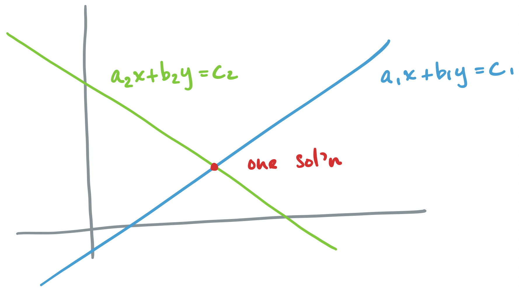
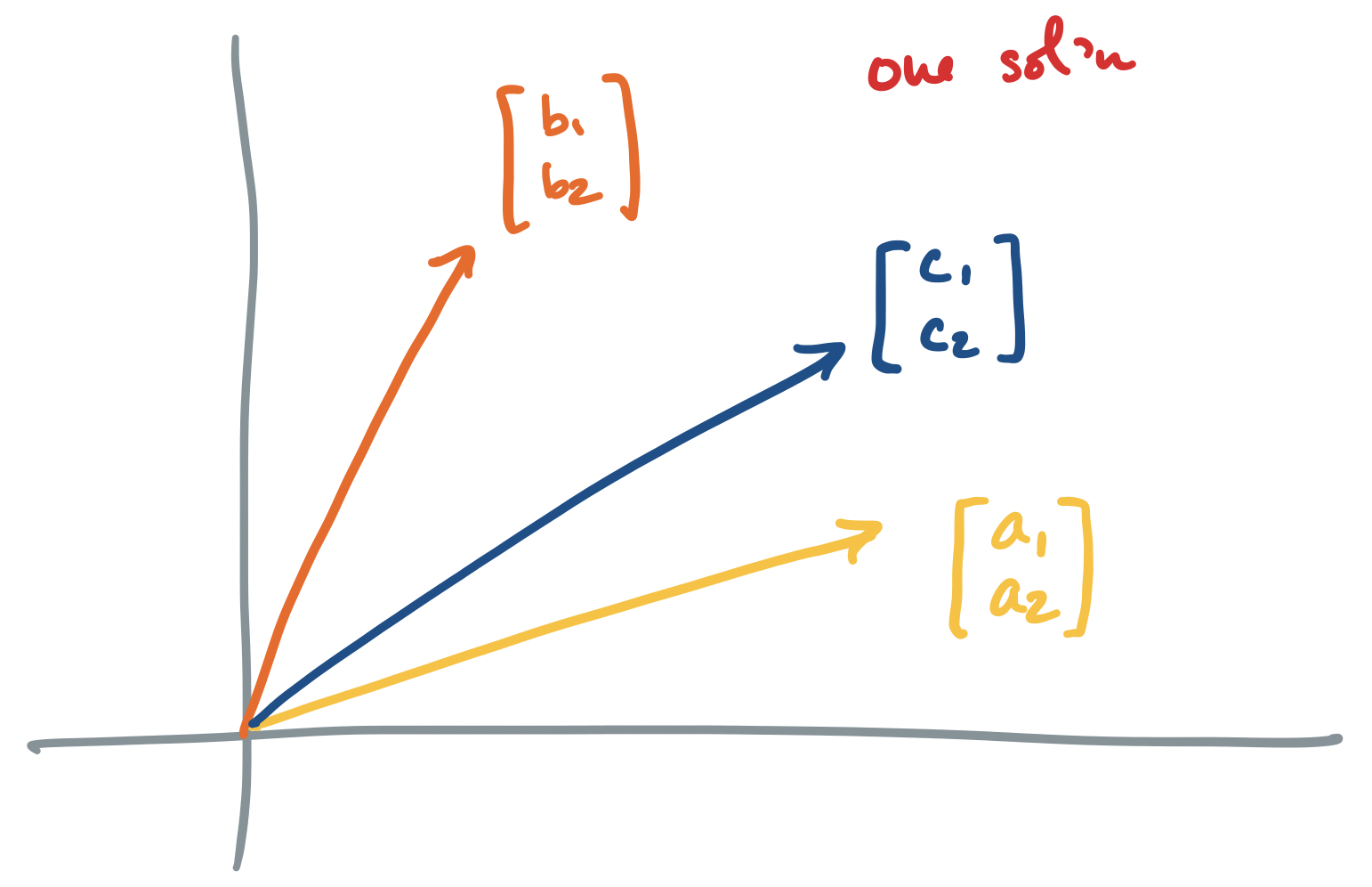
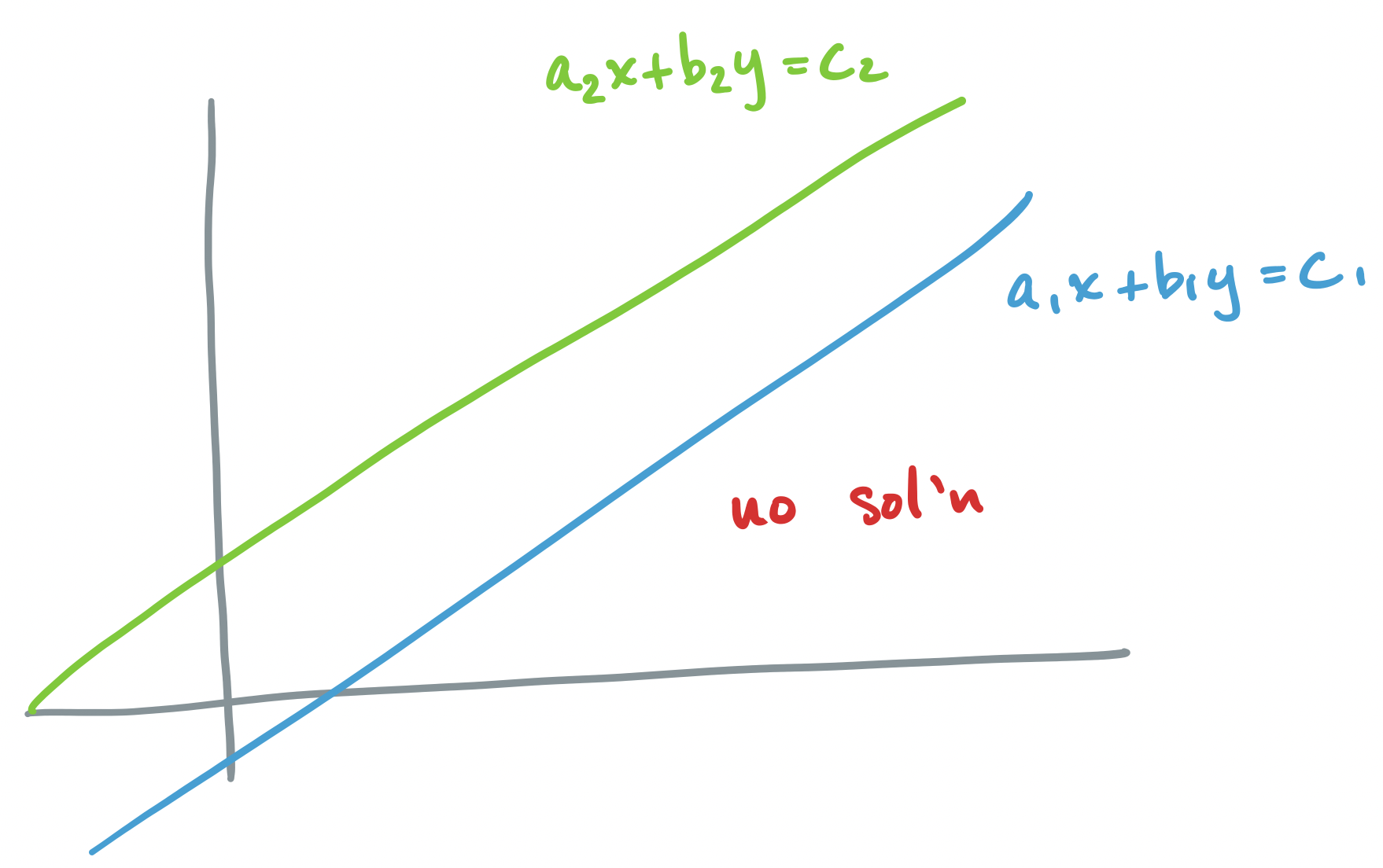
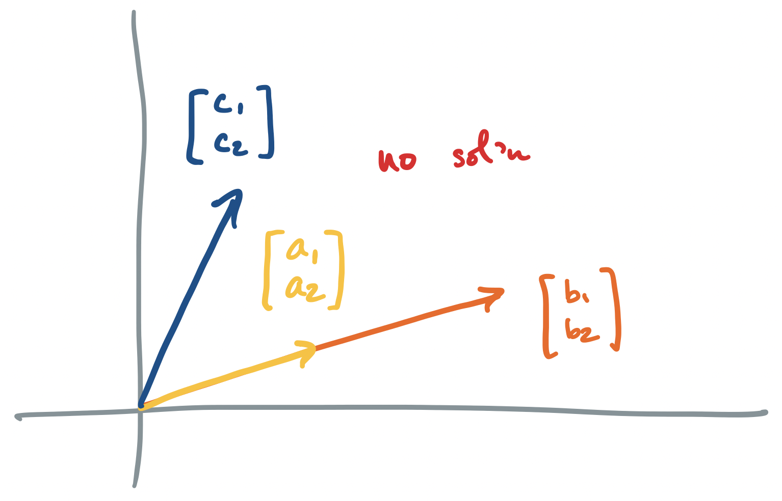
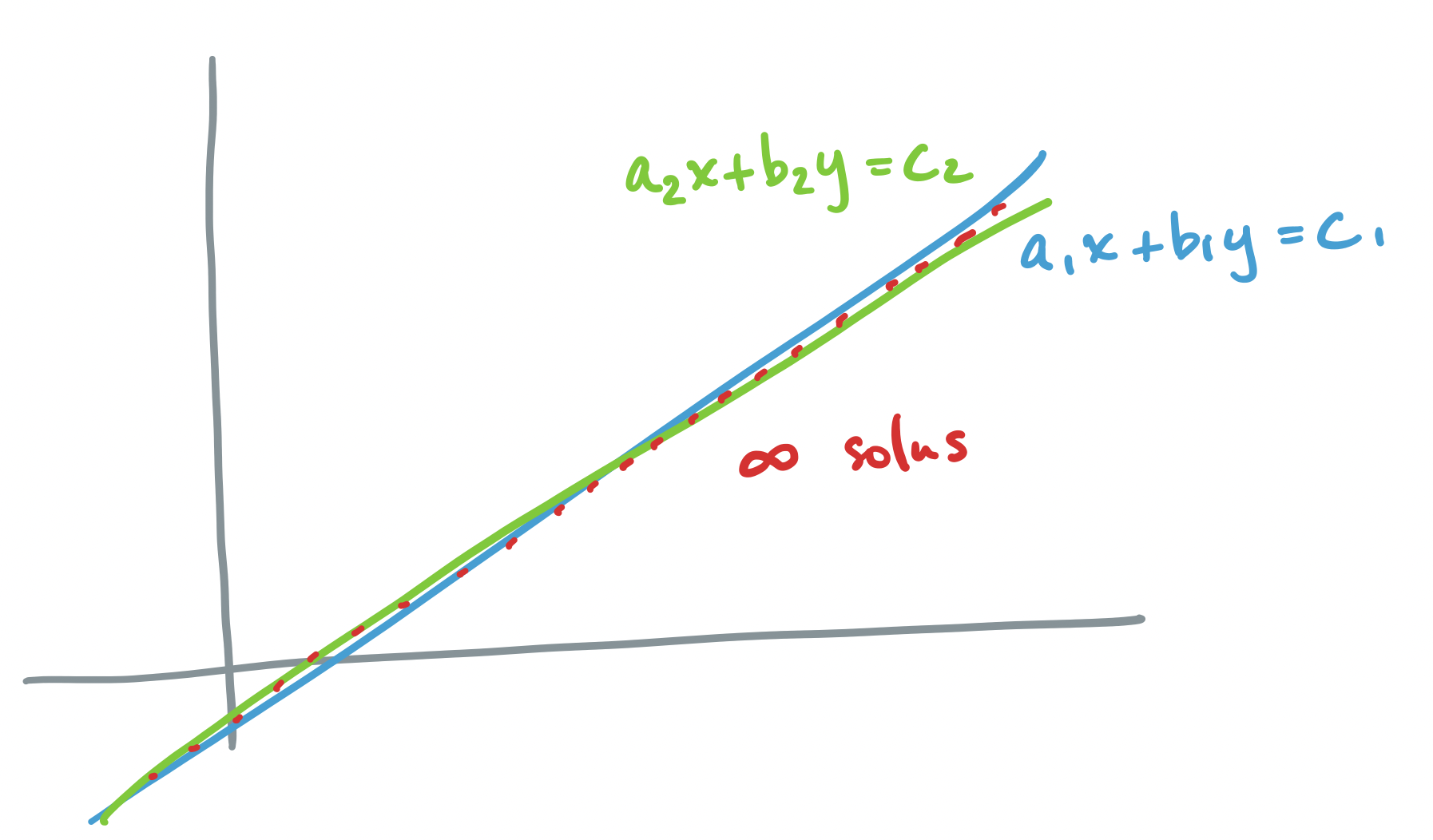
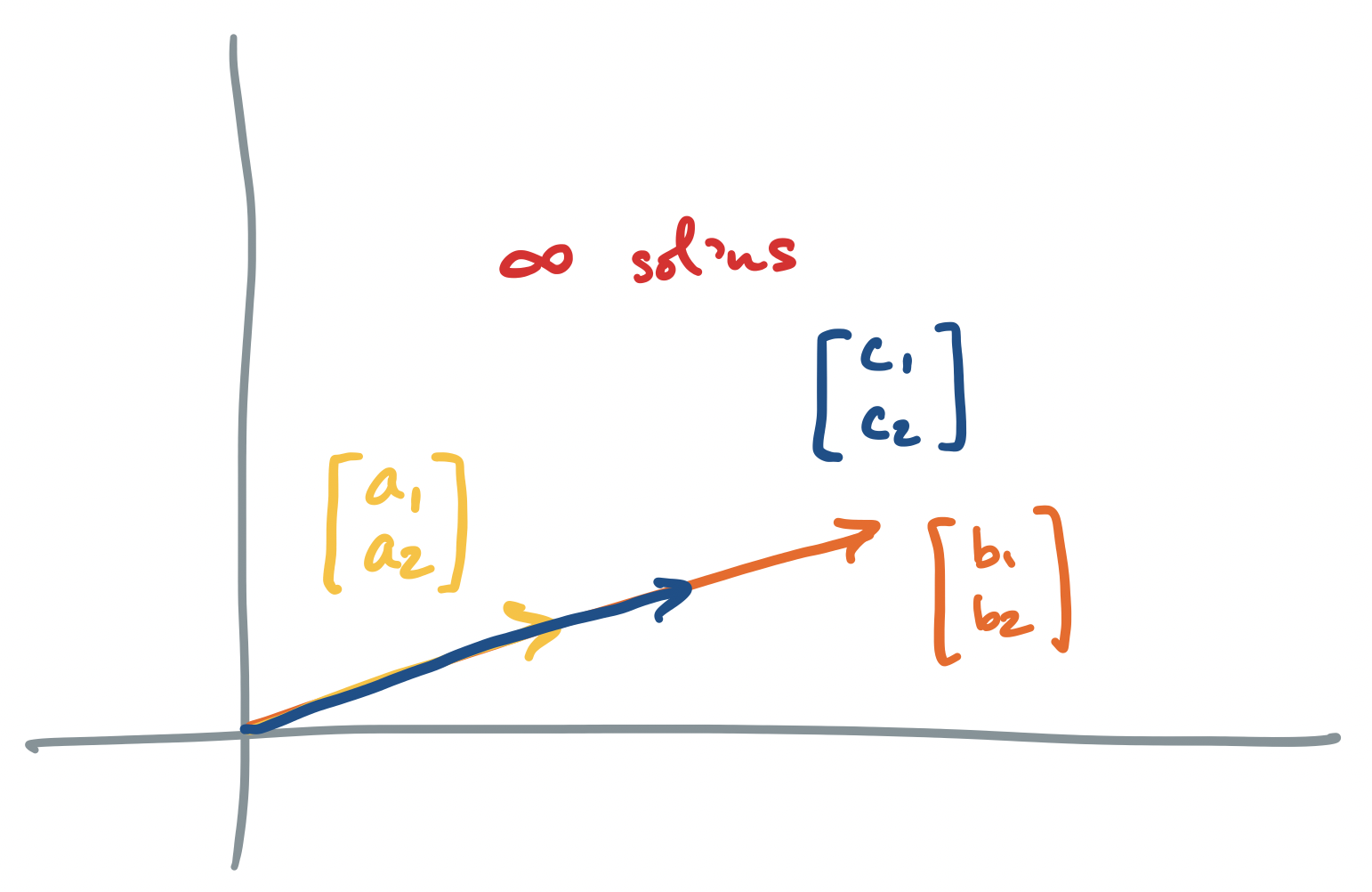
Let's go through each scenario described above, for the system $A \mathbf x = \mathbf b$ where $A = \begin{bmatrix} a_1 & b_1 \\ a_2 & b_2 \end{bmatrix}$ and $\mathbf b = \begin{bmatrix} c_1 \\ c_2 \end{bmatrix}$.
-
If $A\mathbf x = \mathbf b$ has exactly one solution, the geometric interpretation says that there is exactly one point at which all of our equations intersect. The corresponding vector interpretation is that of linearly independent vectors for which there exists one linear combination to describe $\mathbf b$.
-
If $A \mathbf x = \mathbf b$ has no solution, we said above that the vector interpretation says that there are no linear combinations of our column vectors that produces $\mathbf b$. The traditional geometric interpretation describes two objects (lines, planes, etc) which do not intersect.
-
If $A \mathbf x = \mathbf b$ has infinitely many solutions, we said above that we have linearly dependent columns. So the vector interpretation says that we have infinitely many ways to combine our column vectors to produce $\mathbf b$. The geometric interpretation describes two objects (lines, planes, etc) which intersect along at least a line, but maybe even a plane or more in higher dimensions. Since lines are infinitely long, there are infinitely many intersection points.
Again, what is the data story here? As discussed earlier, one thing we would like to do when treating our dataset as a matrix is to identify those vectors that can be described as linear combinations of the columns. In this way, we get information about the relationship of the new vector with our existing dataset. The three scenarios we get then are:
- we can describe the new vector perfectly as an exact linear combination of the existing data,
- the new vector cannot be described at all by the existing data and lies outside of it, or
- the new vector can be described by some combination of the existing data in many different ways.
As with linear systems, the first occurs when we have a perfect view of our data. It is the other two scenarios that are more realistic. But for now, our goal is to figure out which scenario we're in and what to do in each.