


As mentioned before, the SVD gives us a way to losslessly compress a matrix. By lossless, we mean that the original matrix can be reconstructed perfectly.
However, lossless compression is not viable or necessary in many cases. Much of the digital media we use is compressed lossily: the most widely used image, audio, and video compression algorithms are lossy. The idea behind lossy compression is that exact replication is not necessary because much of the detail that is lost is either undetectable or is just noise.
In some sense, this ties back into the idea of information theory viewed through the lens of machine learning. Machine learning is all about mechanistically trying to find regularities and structure in data. The goal of this is to be able to acquire a simpler description. Such a description is compression in information theoretic terms.
Section 7.2 of the textbook discusses a direct application of this idea: image compression. Recall that images can be represented using matrices. This directly leads us to using rank-$k$ approximations to compress an image.
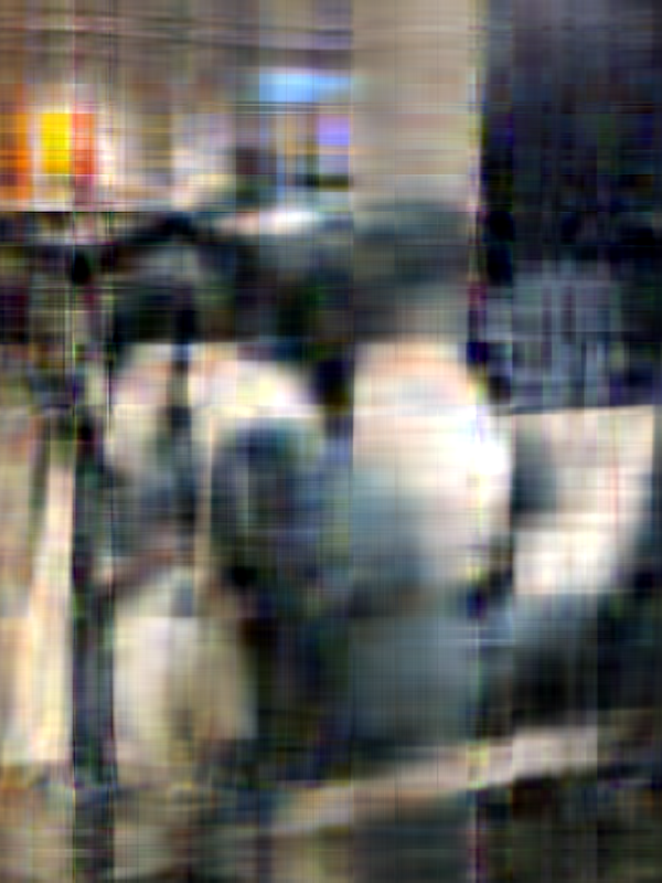
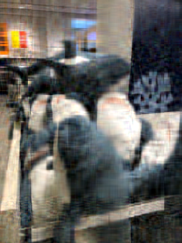
The following images are of the same photo of a pile of Blåhaj at IKEA Shibuya. The original is at the bottom right. From the top left, we have the rank 1, 10, 20, 100, and 200 approximations obtained via SVD.
It's hard to see at the current size on this page, but if you view the images at their actual size, you'll see that there is still a slight but noticeable difference between the rank 100 approximation and the rank 200 approximation, but the rank 200 approximation is virtually indistinguishable from the original.
How does this work? Recall that an image is a grid of pixels and each pixel is a 3-tuple $(R, G, B)$ specifying a red, green, and blue component. The simplest version of this treats each component as an unsigned 8-bit integer, which ranges from 0 to 255. The idea is to obtain three matrices: one for the red values, one for greens, and one for blues. We perform SVD on each of these matrices, take the rank $k$ approximation of each, and put them together to get the compressed image.
    # read image
    img = plt.imread("my-image.png")

    # extract component matrices
    rs = img[:,:,0]
    gs = img[:,:,1]
    bs = img[:,:,2]

    # get svd for each component
    ur,sr,vtr = np.linalg.svd(rs)
    ug,sg,vtg = np.linalg.svd(gs)
    ub,sb,vtb = np.linalg.svd(bs)

    k = 5    # set desired rank

    # compose the rank k approximation
    # note that svd may take values outside of range
    # need to cast to uint8
    rk = np.uint8(ur[:,:k] * sr[:k] @ vtr[:k])
    gk = np.uint8(ug[:,:k] * sg[:k] @ vtg[:k])
    bk = np.uint8(ub[:,:k] * sb[:k] @ vtb[:k])

    # put all the matrices together to form image
    compressed_img = np.dstack((rk,gk,bk))
One can compute approximately how good this compression is based on the sizes of the matrices. The original photo, taken on an iPhone 8, was very large, something like 4000 by 3000-ish pixels (i.e. 12 megapixels). For this exercise, I scaled the original down to 600 by 800 first and used that as the starting point. Such an image results in a matrix of rank 600.
| Rank | Expression | Size | Ratio |
|---|---|---|---|
| 600 | $600 \times 800$ | 480000 | 1 |
| 1 | $600 \times 1 + 1 + 1 \times 800$ | 1401 | 340 |
| 10 | $600 \times 10 + 10 + 10 \times 800$ | 14010 | 34 |
| 20 | $600 \times 20 + 20 + 20 \times 800$ | 28020 | 17 |
| 100 | $600 \times 100 + 100 + 100 \times 800$ | 140100 | 3.4 |
| 200 | $600 \times 200 + 200 + 200 \times 800$ | 280200 | 1.7 |
As with any compression method, the effectiveness depends on the amount of regularities in the original image. For instance, images that are flatter and with fewer colours are easier to compress and more complex images will be more difficult to compress.
Principal Component Analysis is a technique that has its origins in statistics. This is not a statistics class. Instead, like linear regression, we'll view it structurally. In this view, the basic idea of PCA is to find a low-dimensional representation or description (i.e. some subspace) for some data that we have. Obviously, we would like such a description to have minimal error. For a dataset $\mathbf a_1, \dots, \mathbf a_n$, this is done by minimizing the distances of all $\mathbf a_i$ to such a subspace. The goal of PCA is to find an orthonormal basis $\mathbf q_1, \dots, \mathbf q_k$ for this "best $k$-dimensional subspace of fit".
This sounds suspiciously similar to the least squares linear regression we were doing a few weeks ago. It's not entirely off-base: linear regression is also trying to find a low-dimensional subspace of best fit. But there's a subtle difference in what the two methods are trying to accomplish. Suppose we have the following dataset.
| $t$ | $b$ |
|---|---|
| -12 | 8 |
| -2 | -7 |
| 1 | 9 |
| 4 | -13 |
| 9 | 3 |
First, let's think about what such a basis would look like with respect to our dataset. What we want to do is to minimize all of the distances from every $\mathbf a_i$ to their projections onto our subspace. The orthogonality of our basis is helpful in this case: this means all we need is to consider the projections onto each dimension, one at a time, because they don't "interfere" with each other.
Again, we note that this differs from least squares regressions, which seeks to compute $\mathbf x$ so that it minimizes $\|A \mathbf x - \mathbf b\|^2$. Instead, we try to find a basis vector that minimizes $\|\mathbf e\|^2$, the error term or in this case, the distance between $\mathbf a_i$ and its projection onto the subspace described by the basis vector.
If we draw the lines that we find, we see that they are quite different:
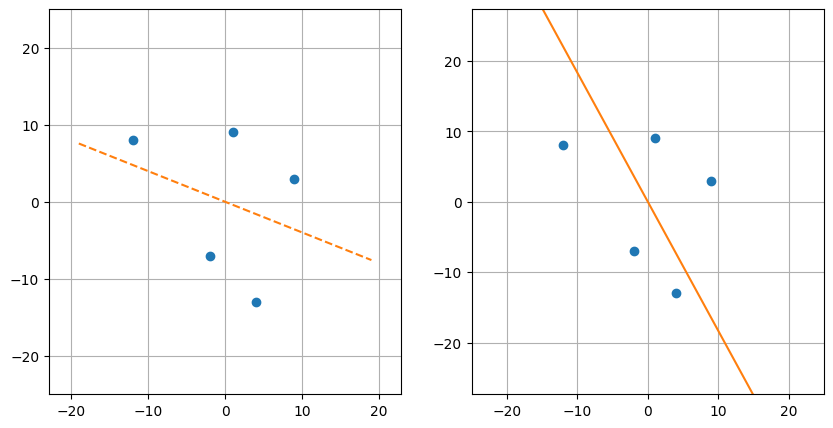
On the left is the view of least squares: minimizing the "vertical" distance to the line of best fit. On the right is view of principal component analysis: minimizing the distance to the "direction" of best fit—this is perpendicular rather than vertical. What's the difference? In the case of regression, only the distance concerning the target variable (i.e. the vertical distance) matters, while in PCA, the distance over the entire space matters.
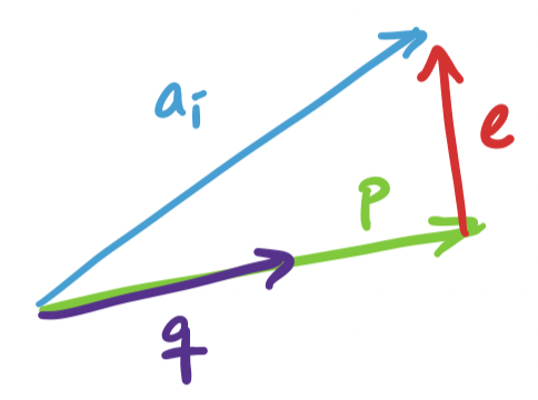
Since we can break up our search for $k$ basis vectors into one dimension at a time, we can consider the one dimensional case, where we project $\mathbf a_i$ onto some unit vector $\mathbf q$. This projection is $\mathbf p = \mathbf q \mathbf q^T \mathbf a_i$. We have ourselves a right triangle again and we see that the lengths work out so that we have
\[\|\mathbf a_i\|^2 = \|\mathbf q \mathbf q^T \mathbf a_i\|^2 + \|\mathbf e\|^2.\]
This is the projection problem except almost in reverse. In the projection problem, the subspace described by the basis $\mathbf a$ is fixed and we're trying to project $\mathbf b$ onto $\mathbf a$. But in PCA, the vector $\mathbf a_i$ we're trying to project is fixed (because it's the data) and it's the subspace or basis vector $\mathbf q$ that we're trying to find. In both cases, the goal is to minimize $\|\mathbf e \|^2$.
Since $\mathbf a_i$ is fixed, our only choice is to find $\mathbf q$ so that $\|\mathbf q \mathbf q^T \mathbf a_i\|^2$ is as large as possible. What exactly is this quantity? Recall that $\mathbf q^T \mathbf a_i$ is the dot product $\mathbf q \cdot \mathbf a_i$. This means we can view $\mathbf q \mathbf q^T \mathbf a_i$ as $(\mathbf q \cdot \mathbf a_i)\mathbf q$, a scalar multiple of $\mathbf q$. Since $\|\mathbf q\| = 1$, the length of the resulting projection is exactly $\mathbf q \cdot \mathbf a_i$, making $\|\mathbf p\| = (\mathbf q \cdot \mathbf a_i)^2$.
Now, suppose we have all of our $\mathbf a_i$'s in a single matrix $A$. To compute $(\mathbf q \cdot \mathbf a_i)^2$ for all of these at the same time, we have \[\sum_{i=1}^n (\mathbf a_i \cdot \mathbf q)^2 = (A\mathbf q)^T (A \mathbf q) = \mathbf q^T A^T A \mathbf q.\] Again, recall that $A$, which contains our dataset is fixed, which must mean that what we need to do is try to find $\mathbf q$ that maximizes the quantity above. But in fact, we've already seen this quantity show up before: it's $\|A\mathbf q\|^2$.
However, this time we can say more, since we know that $A^TA = V \Sigma^2 V^T$. Let's consider what happens when we take $\mathbf q^T V \Sigma^2 V^T \mathbf q$. Since $V$ is orthogonal, the length of $\mathbf q$ doesn't get changed by $V$. That is $\|V \mathbf q\| = \|\mathbf q\|$. However, $\Sigma^2$ does change its length: it "stretches" the vector according to its linear combination by $V$. After this stretching, its length doesn't change again since $\|\mathbf q\| = 1$.
This coincides with our understanding of unit vectors undergoing a transformation through $A^TA$ as having length that "averages" the eigenvalues $\sigma_i^2$. So it seems that to maximize this value, we need to maximize the involvement of the eigenvector with the largest eigenvalue. By convention, this eigenvector is $\mathbf v_1$, which has eigenvalue $\sigma_1^2$.
The result is that the vector $\mathbf q$ that maximizes $\mathbf q^T A^TA \mathbf q$ is $\mathbf v_1$, the first singular vector. And we have already seen before that \[\|A \mathbf v_1\|^2 = \lambda_1 = \sigma_1^2.\]
What we need to show now is that any other unit vector $\mathbf q$ gives us $\mathbf q^T A^TA \mathbf q \leq \sigma_1^2$. Notice that this leads us directly to the spectral norm. If we want to generalize this argument for any vector $\mathbf x$, we need to consider the length of $\mathbf x$. This is easy: just normalize it. So we have \[\frac{\mathbf x^T}{\|\mathbf x\|} A^T A \frac{\mathbf x}{\|\mathbf x\|} = \frac{\mathbf x^T A^T A \mathbf x}{\|x\|^2} = \frac{\|A\mathbf x\|^2}{\|\mathbf x\|^2} \leq \sigma_1^2,\] which gives us $\frac{\|A \mathbf x\|}{\|\mathbf x\|} \leq \sigma_1$ for all nonzero vectors $\mathbf x$.
Since we assume we want an orthonormal basis (and this guarantees that we will get one by the diagonalization of $A^TA$), we simply repeat this process for each successive dimension: the next vector that maximizes the next direction will be $\mathbf v_2$, and so on. What we find is exactly what we want: the principal components are the vectors associated with the largest singular vectors.
So we've seen that SVD gives us PCA almost for free. The other side of the coin is that PCA confirms that SVD does indeed give us the best rank $k$ approximation of $A$, by convincing us that the principal components coincide with the singular vectors associated with the largest singular values.
Let's think back to the beginning of the quarter. We had this notion of vectors as objects that could be added together and scaled. These represent objects or data. Since they're finite dimensional, we can focus our attention on $\mathbb R^n$ (things would be a bit different if we considered infinite-dimensional vector spaces).
We are concerned with collections of data, which means we need to work with collections of vectors. Such objects are matrices. Like vectors, we can combine matrices in certain ways, the most significant of which was via matrix multiplication. Matrix multiplication was already enough to lead to our first example: the recommendation system. This was the setup in which our matrix $A$ contained ratings of products by users, with each column representing a user profile and each row representing a product.
At the time, we had the following observations.
All of this was achieved simply through understanding the mechanism of matrix multiplication. This led to the following questions:
These are questions that involve ideas about linear independence, vector spaces, and bases. Over the course of the course, we got some answers.
But there's a problem:
The singular value decomposition and low-rank approximations close the loop on these questions. SVD combines everything that we've done in the course to give us a way out:
Notice the work required to get here:
These are the basic ingredients for working with matrices and linear data. And these are the basic ideas that machine learning algorithms and data analysis techniques exploit to uncover the latent structures laying hidden inside data. Obviously, there are many more sophsiticated approaches and techniques out there, but they all build on a basic understanding of these fundamental pieces.