When we first started our discussion of eigenvectors, we learned that only square matrices had them. However, we just saw something very interesting: if we take an arbitrary $m \times n$ matrix, then the eigenvectors of $A^TA$ and $AA^T$ turn out to contain an orthogonal basis for all four subspaces of $A$. Ideally, we would want to put these two sets of vectors together. To do that, we examine the eigenvalues of $A^TA$ and $AA^T$. In doing so, we notice that the two sets of eigenvalues contain the same non-zero eigenvalues.
For any $m \times n$ matrix $A$, the matrices $A^TA$ and $AA^T$ have the same non-zero eigenvalues.
Consider an eigenvector $\mathbf v$ of $A^TA$ and suppose its eigenvalue is $\lambda$. Then $A^TA \mathbf v = \lambda \mathbf v$. Multiplying both sides by $A$, we get: \begin{align*} A(A^TA \mathbf v) &= A(\lambda \mathbf v) \\ AA^T(A \mathbf v) &= \lambda (A \mathbf v) \end{align*} So $A \mathbf v$ is an eigenvector of $AA^T$ with eigenvalue $\lambda$. This relationship works for any eigenvector and eigenvalue of $A^TA$. We can use the exact same argument for $AA^T$.
As an aside, notice that this same argument works for any matrices $A$ and $B$: the products $AB$ and $BA$ will share the same non-zero eigenvalues (assuming they can be multiplied both ways in the first place).
Now that we know that $A^TA$ and $AA^T$ share the same nonzero eigenvalues, one of the consequences is that the eigenvectors with the same eigenvalue must be related to each other.
Let $\mathbf v$ be a unit length eigenvector of $A^TA$ with eigenvalue $\lambda$. Then there is a unit length eigenvector $\mathbf u$ of $AA^T$ with eigenvalue $\lambda$ such that $\mathbf u = \frac{1}{\sqrt{\lambda}} A \mathbf v$.
We know from the previous proof that if $\mathbf v$ is an eigenvector of $A^TA$ with eigenvalue $\lambda$, then $A \mathbf v$ is an eigenvector of $AA^T$ with eigenvalue $\lambda$. So we need to normalize $A \mathbf v$. Recall that since $A^TA$ is positive semidefinite, we have that $\lambda = \frac{\|A \mathbf v\|^2}{\|\mathbf v \|^2}$. But since $\mathbf v$ is unit length, we have $\|\mathbf v\|^2 = 1$ so $\lambda = \|A \mathbf v\|^2$ and therefore $\|A\mathbf v\| = \sqrt \lambda$. This gives us $\frac{A \mathbf v}{\|A \mathbf v\|} = \frac{A \mathbf v}{\sqrt \lambda}$.
Here is our example from last class.
    >>> A = np.array([[ 1,  3,  1,  0,  9],
    ...               [ 0,  0,  0,  1,  3],
    ...               [ 1,  3,  1,  1, 12]])
    >>> L, V = np.linalg.eigh(A.T @ A)
    >>> LL, U = np.linalg.eigh(A @ A.T)
    >>> L
    array([-1.53193879e-14,  2.75212336e-16,  1.12037323e-14,  2.24038498e+00,
            2.55759615e+02])
    >>> LL
    array([-1.77655138e-15,  2.24038498e+00,  2.55759615e+02])
    >>> (A @ V[:,[-1]]) / L[-1]**0.5
    array([[-0.59749492],
           [-0.18317563],
           [-0.78067055]])
    >>> U[:,[-1]]
    array([[-0.59749492],
           [-0.18317563],
           [-0.78067055]])
The consequence of this is that each eigenvector of $A^TA$ can be paired with an eigenvector of $AA^T$ with the same nonzero eigenvalue. We have the following definitions.
Let $\lambda \gt 0$ be a non-zero eigenvalue of $A^TA$ and $AA^T$, $\mathbf v$ be a unit length eigenvector of $A^TA$ with eigenvalue $\lambda$, $\mathbf u$ be a unit length eigenvector of $AA^T$, and $\sigma = \sqrt \lambda$ such that $\mathbf u = \frac 1 \sigma A \mathbf v$.
Here, we note that the left and right singular vectors, which are the eigenvectors of $A^TA$ and $AA^T$, are tied together by their singular values, which are the square roots of the eigenvalues of $A^TA$ and $AA^T$. Though we have shown that $\mathbf u = \frac 1 \sigma A \mathbf v$, we more typically express the relationship as \[A \mathbf v = \sigma \mathbf u,\] which is evocative of the eigenvector equation $A\mathbf x = \lambda \mathbf x$.
Putting all this together, we get the following important result.
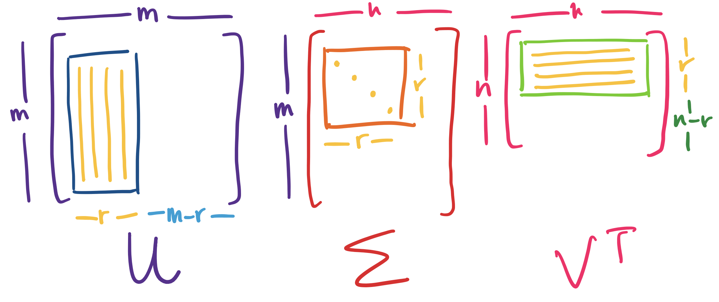
Let $A$ be an $m \times n$ matrix of rank $r$. Then \[A = U \Sigma V^T,\] where $U$ is an orthogonal $m \times m$ matrix, $\Sigma$ is an $m \times n$ diagonal matrix, and $V$ is an orthogonal $n \times n$ matrix.
This factorization of $A$ is called the singular value decomposition of $A$.
Let's dissect this.
Visually, we have the following picture:
Notice that this means
Let's see that this actually works out. First, we mostly have the matrices $U$ and $V$ but we just need to put the columns in the right order. Then we need to set up $\Sigma$.
    >>> A = np.array([[ 1,  3,  1,  0,  9],
    ...               [ 0,  0,  0,  1,  3],
    ...               [ 1,  3,  1,  1, 12]])
    >>> L, U = np.linalg.eigh(A @ A.T)
    >>> _, V = np.linalg.eigh(A.T @ A)
    >>> S = np.zeros((3,5))
    >>> np.fill_diagonal(S, L[::-1] ** 0.5)
    RuntimeWarning: invalid value encountered in sqrt np.fill_diagonal(S, L[::-1] ** 0.5)
    >>> S
    array([[15.99248621,  0.        ,  0.        ,  0.        ,  0.        ],
           [ 0.        ,  1.49679156,  0.        ,  0.        ,  0.        ],
           [ 0.        ,  0.        ,         nan,  0.        ,  0.        ]])
Here, we set up $\Sigma$. We note that numpy.linalg.eigh will give eigenvalues in increasing order, so we just have to reverse everything. Notice that the singular values are the square roots of the eigenvalues of $A^TA$ and $AA^T$. However, because some zeros can come up as a small amount of negative error, we may need to fix this.
    >>> S[2,2] = 0
    >>> S
    array([[15.99248621,  0.        ,  0.        ,  0.        ,  0.        ],
           [ 0.        ,  1.49679156,  0.        ,  0.        ,  0.        ],
           [ 0.        ,  0.        ,  0.        ,  0.        ,  0.        ]])
    >>> U = U[:,::-1]
    >>> V = V[:,::-1]
    >>> U @ S @ V.T
    array([[ 1.00000000e+00,  3.00000000e+00,  1.00000000e+00,
             1.22124533e-15,  9.00000000e+00],
           [ 3.44169138e-15, -6.99440506e-15, -1.66533454e-16,
             1.00000000e+00,  3.00000000e+00],
           [ 1.00000000e+00,  3.00000000e+00,  1.00000000e+00,
             1.00000000e+00,  1.20000000e+01]])
That's a bit hard to read, so let's round.
    >>> np.round(U @ S @ V.T)
    array([[ 1.,  3.,  1.,  0.,  9.],
           [ 0., -0., -0.,  1.,  3.],
           [ 1.,  3.,  1.,  1., 12.]])
So we have computed the SVD of $A$ by computing the eigenvectors and eigenvalues of $A^TA$ and $AA^T$, thereby verifying the relationship between all of these pieces. Luckily, we don't actually need to do this to compute the SVD: the function numpy.linalg.svd will produce $U, \Sigma, V$ for you, though there are some details to be aware of.
    >>> A = np.array([[ 1,  3,  1,  0,  9],
    ...               [ 0,  0,  0,  1,  3],
    ...               [ 1,  3,  1,  1, 12]])
    >>> U, S, Vt = np.linalg.svd(A)
    >>> S
    array([1.59924862e+01, 1.49679156e+00, 7.52107468e-16])
    >>> U
    array([[-0.59749492,  0.55647685, -0.57735027],
           [-0.18317563, -0.7956842 , -0.57735027],
           [-0.78067055, -0.23920735,  0.57735027]])
    >>> Vt
    array([[-0.08617581, -0.25852743, -0.08617581, -0.06026869, -0.95638837],
           [ 0.21196639,  0.63589917,  0.21196639, -0.69140659, -0.16652227],
           [ 0.96666102, -0.09059904, -0.13822101,  0.18554763, -0.06184921],
           [-0.06901933,  0.67792842,  0.09904226,  0.68793606, -0.22931202],
           [-0.09190644,  0.24698317, -0.95850381, -0.10315358,  0.03438453]])
Here are the caveats to keep mind:
Something that was guiding our discussion of eigenvectors was the view of an $n \times n$ matrix $A$ as a transformation of vectors in $\mathbb R^n$. How does that relate to transformations of vectors from $\mathbb R^n$ to $\mathbb R^m$, as is in $m \times n$ matrices? That we can take a vector and transport it from $\mathbb R^n$ to $\mathbb R^m$ seemed a bit like science fiction. However, we are now able to get a more detailed breakdown of this process via the SVD: if $A = U \Sigma V^T$, then the transformation $A$ can be viewed as a transformation $V^T$, followed by $\Sigma$, followed by $U$.
First, we recall a key observation: orthogonal matrices only rotate vectors. How do we know this? Recall that the determinant of any orthogonal matrix $Q$ is $\pm 1$. Intuitively, the "volume" doesn't change after transformation under $Q$ since the basis vectors don't scale. This gives us the following breakdown:
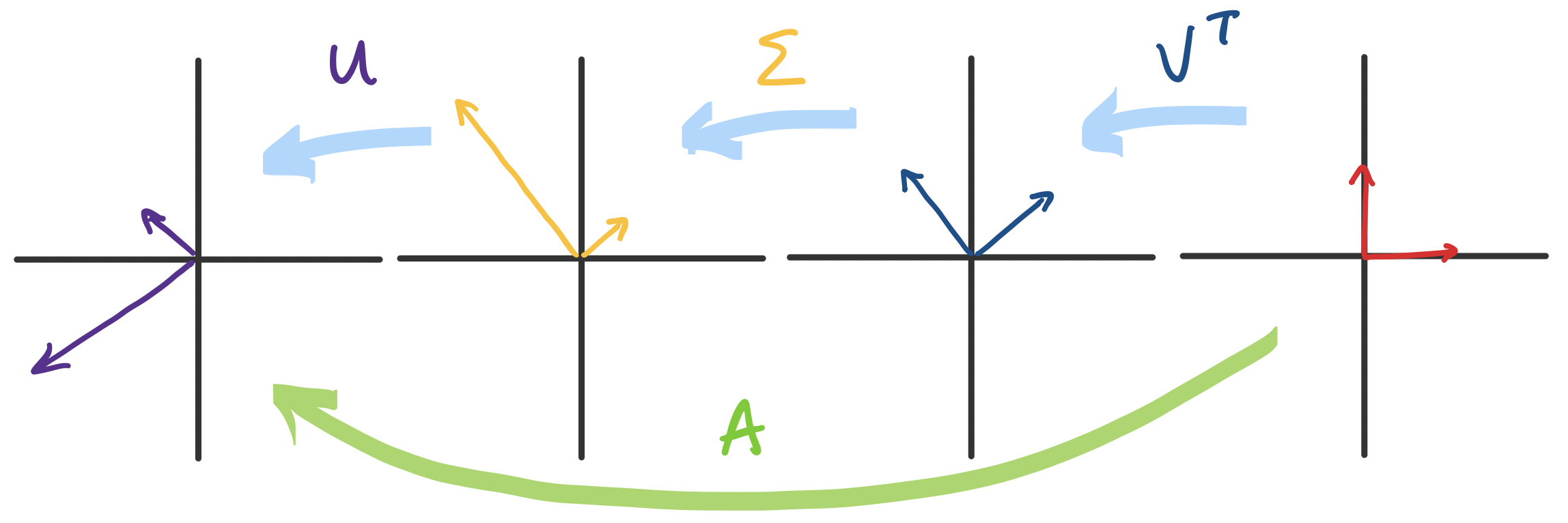
There are some interesting things to note here:
This last point is actually quite important and gives us the final piece of the puzzle in understanding the latent structures in matrices. Recall that the singular values of any matrix are nonnegative and have associated singular vectors. This means that each singular value defines a "piece" of the matrix. This piece has an associated direction and basis vector: the singular vectors.
Recall that we can view a matrix product $AB$ as a sum of rank one products: \[\begin{bmatrix} \quad \\ \mathbf a_1 & \mathbf a_2 & \cdots & \mathbf a_n \\ \quad \end{bmatrix} \begin{bmatrix} \quad & \mathbf b_1 & \quad \\ & \mathbf b_2 \\ & \vdots \\ & \mathbf b_n \end{bmatrix} = \mathbf a_1 \mathbf b_1 + \mathbf a_2 \mathbf b_2 + \cdots + \mathbf a_n \mathbf b_n.\] In our case, we have \begin{align*} U \Sigma V^T &= \begin{bmatrix} \quad \\ \mathbf u_1 & \mathbf u_2 & \cdots & \mathbf u_m \\ \quad \end{bmatrix} \begin{bmatrix} \sigma_1 & & & \\ & \sigma_2 \\ && \ddots \\ &&& \sigma_{\min\{m,n\}} \end{bmatrix} \begin{bmatrix} \quad & \mathbf v_1^T & \quad \\ & \mathbf v_2^T \\ & \vdots \\ & \mathbf v_n^T \end{bmatrix} \\ &= \mathbf u_1 \sigma_1 \mathbf v_1^T + \mathbf u_2 \sigma_2 \mathbf v_2^T + \cdots + \mathbf u_{\min\{m,n\}} \sigma_{\min\{m,n\}} \mathbf v_{\min\{m,n\}} ^T \\ &= \sigma_1 \mathbf u_1 \mathbf v_1^T + \sigma_2 \mathbf u_2 \mathbf v_2^T + \cdots + \sigma_{\min\{m,n\}} \mathbf u_{\min\{m,n\}} \mathbf v_{\min\{m,n\}} ^T \end{align*}
Visually, we can view each term as being put together using the following pieces:
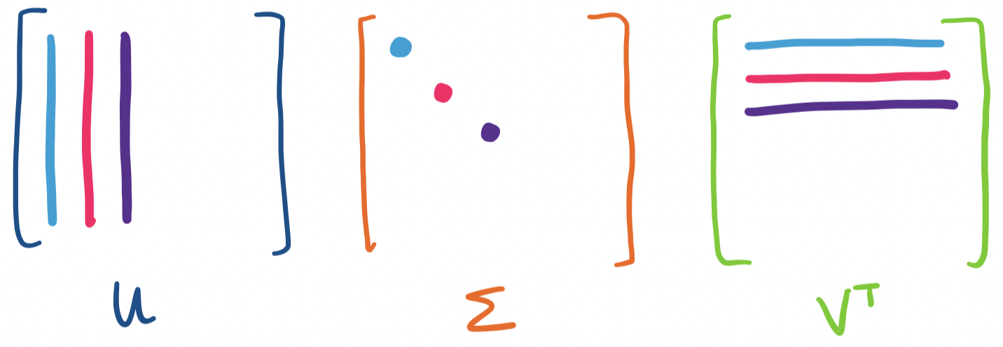
Now, recall that all of the singular vectors have length 1, which means any outer product is going to result in entries less than 1. This makes the scaling by the singular value extremely important. But since singular values are ordered from greatest to least, this suggests that the directions associated with the largest singular values are going to have the most "weight" in this sum. In other words, these are the dominant directions of the matrix.
Let's look at the rank 1 matrices corresponding to each singular value.
    >>> S[0,0]
    15.99248621
    >>> S[1,1]
    1.49679156
    >>> S[0,0] * U[:,[0]] @ V[:,[0]].T
    array([[ 0.82344686,  2.47034059,  0.82344686,  0.5758932 ,  9.13870137],
           [ 0.25244633,  0.757339  ,  0.25244633,  0.17655314,  2.80167641],
           [ 1.0758932 ,  3.22767959,  1.0758932 ,  0.75244633, 11.94037778]])
    >>> S[1,1] * U[:,[1]] @ V[:,[1]].T
    array([[ 0.17655314,  0.52965941,  0.17655314, -0.5758932 , -0.13870137],
           [-0.25244633, -0.757339  , -0.25244633,  0.82344686,  0.19832359],
           [-0.0758932 , -0.22767959, -0.0758932 ,  0.24755367,  0.05962222]])
Notice that, the first piece is larger, since it's scaled/weighted by a larger singular value.
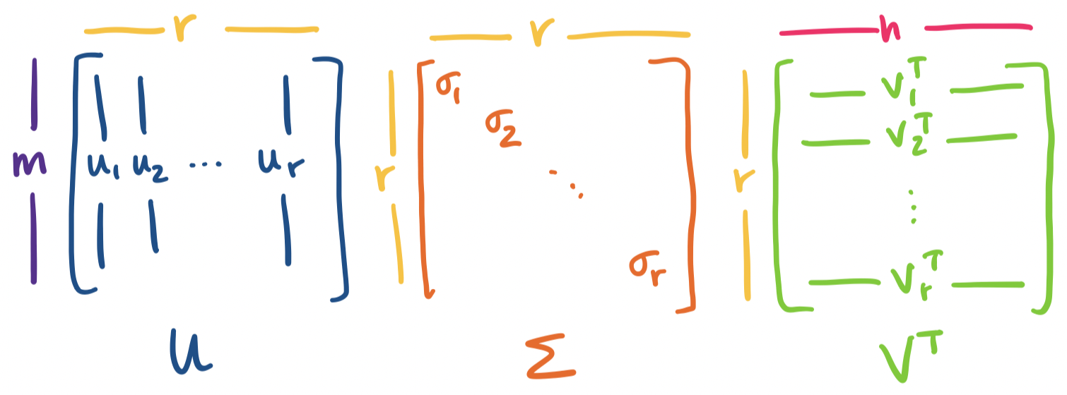
Now, suppose $A$ has rank $r \lt m,n$. In this case, $A$ has $r$ nonzero singular values and the rest are 0. So we can simplify the above expression further: \begin{align*} A &= \sigma_1 \mathbf u_1 \mathbf v_1^T + \cdots + \sigma_r \mathbf u_r \mathbf v_r^T + \sigma_{r+1} \mathbf u_{r+1} \mathbf v_{r+1}^T + \cdots + \sigma_{\min\{m,n\}} \mathbf u_{\min\{m,n\}} \mathbf v_{\min\{m,n\}}^T\\ &= \sigma_1 \mathbf u_1 \mathbf v_1^T + \cdots + \sigma_r \mathbf u_r \mathbf v_r^T + 0 + \cdots + 0 \\ &= \sigma_1 \mathbf u_1 \mathbf v_1^T + \cdots + \sigma_r \mathbf u_r \mathbf v_r^T \end{align*}
So in fact, we only need first $r$ singular values and their singular vectors to completely describe $A$. If we put these into a matrix, this gives us an $m \times r$ matrix $U$, an $r \times r$ matrix $\Sigma$, and an $n \times r$ matrix $V$. This is often called the reduced SVD.
We add the two pieces from our previous example, since $A$ has rank 2:
    >>> np.round(S[0,0] * U[:,[0]] @ V[:,[0]].T + S[1,1] * U[:,[1]] @ V[:,[1]].T)
    array([[ 1.,  3.,  1.,  0.,  9.],
           [ 0., -0., -0.,  1.,  3.],
           [ 1.,  3.,  1.,  1., 12.]])
Of course, this is equivalent to just taking the matrices containing only the respective singular values and vectors and taking their product.
    >>> np.round(U[:,:2] @ S[:2,:2] @ V[:,:2].T)
    array([[ 1.,  3.,  1.,  0.,  9.],
           [ 0., -0., -0.,  1.,  3.],
           [ 1.,  3.,  1.,  1., 12.]])
These pieces comprise the reduced SVD for $A$.
Note that setting the full_matrices parameter of numpy.linalg.svd to False computes the SVD to size $\min\{m,n\}$, not the rank of the matrix. For instance, the rank of $A$ is 2 but:
    >>> U, S, Vt = np.linalg.svd(A, full_matrices=False)
    >>> S
    array([1.59924862e+01, 1.49679156e+00, 7.52107468e-16])
    >>> U
    array([[-0.59749492,  0.55647685, -0.57735027],
           [-0.18317563, -0.7956842 , -0.57735027],
           [-0.78067055, -0.23920735,  0.57735027]])
    >>> Vt
    array([[-0.08617581, -0.25852743, -0.08617581, -0.06026869, -0.95638837],
           [ 0.21196639,  0.63589917,  0.21196639, -0.69140659, -0.16652227],
           [ 0.96666102, -0.09059904, -0.13822101,  0.18554763, -0.06184921]])
The significance of the existence of the SVD is both completely natural and kind of astonishing. It is astonishing because it's actually pretty incredible that such a decomposition that contains evertyhing we want to know about our matrix exists—particularly when all of the decompositions we've seen before require our matrices to have special properties.
And yet, this is a completely natural result. If we believe that matrices have certain structures to them, like the fundamental subspaces, and these structures themselves have properties of their own, then of course there should be a decomposition that exposes these structures.
In a way, the SVD is the natural ending point for the work that we've done in this course:
This last point takes us to the last stop in the course, giving us arguably the most useful piece of the SVD: it gives us a convenient tool to describe large, complex, high-dimensional data by identifying the most important basis directions. This is a fitting conclusion to the theme of the course: decomposing large, complex matrices into simpler, tractable parts that expose the underlying structures.