Eigenvectors present us with another opportunity to decompose a matrix. Suppose first that we happen to have an $n \times n$ matrix $A$ with $n$ independent eigenvectors (not obvious that we can always do this!). We use our usual trick for working with several vectors: make them the columns of a matrix. What do we gain from this?
First, remember that if we have an eigenvector $\mathbf x$, we have that $A \mathbf x = \lambda \mathbf x$. Now, suppose we take each eigenvector $\mathbf x_1, \dots, \mathbf x_n$ and put them in a matrix $X$. What is the matrix product $AX$? If we apply the usual column-centric view of matrix multiplication, we have \[AX= A \begin{bmatrix} \quad \\ \mathbf x_1 & \cdots & \mathbf x_n \\ \quad \end{bmatrix} = \begin{bmatrix} \quad \\ \lambda_1 \mathbf x_1 & \cdots & \lambda_n \mathbf x_n \\ \quad \end{bmatrix}.\] To see why this is the case, recall that the $i$th column of $X$ determines the $i$th column of the product $AX$ and it is equal to $A$ multiplied by that column. In this case, the $i$th column of $X$ is $\mathbf x_i$, so $A \mathbf x_i = \lambda_i \mathbf x_i$.
To get the decomposition we're looking for, we now decompose the right hand side. We have \[\begin{bmatrix} \quad \\ \lambda_1 \mathbf x_1 & \cdots & \lambda_n \mathbf x_n \\ \quad \end{bmatrix} = \begin{bmatrix} \quad \\ \mathbf x_1 & \cdots & \mathbf x_n \\ \quad \end{bmatrix} \begin{bmatrix} \lambda_1 & & \\ & \ddots & \\ & & \lambda_n \end{bmatrix} = X \Lambda.\] This is fairly straightforward: our product is simply the rhs of the eigenvector equation, so we split up the eigenvectors and eigenvalues. We denote the eigenvalue matrix by $\Lambda$, which is the uppercase version of $\lambda$. This gives us the following theorem.
Let $A$ be an $n \times n$ matrix with $n$ linearly independent eigenvectors. Then $AX = X \Lambda$, where $X$ is the matrix of eigenvectors of $A$ and $\Lambda$ is a diagonal matrix of eigenvalues of $A$.
One thing to note here is that $X$ is gives us a basis for the column space of $A$. If the eigenvectors have nonzero eigenvalues, they are in the column space of $A$ (since $A \mathbf x = \lambda \mathbf x)$. If we have $n$ such linearly independent vectors, this gives us a basis.
This gives us a way to satisfy the following definition:
A matrix $A$ is diagonalizable if there exists an invertible matrix $P$ and a diagonal matrix $D$ such that $A = PDP^{-1}$.
So we have that $P = X$, the matrix of eigenvectors, and $D = \Lambda$, the matrix of eigenvalues.
Why is this useful? Remember that a requirement is that $A$ has $n$ linearly independent eigenvectors. This means that the columns of $X$ are all independent—that is, $X$ is invertible. We have the following corollary:
Let $A$ be an $n \times n$ matrix with $n$ linearly independent eigenvectors. Then $A = X \Lambda X^{-1}$ and $\Lambda = X^{-1} A X$.
Consider the matrix $A = \begin{bmatrix} -1 & 0 & -8 \\ 0 & -1 & 8 \\ 0 & 0 & 3 \end{bmatrix}$. Since $A$ is upper triangular, we have that the eigenvalues of $A$ are $-1$ (with multiplicity 2) and $3$.
    >>> A = np.array([[-1, 0, -8], [0, -1, 8], [0, 0, 3]])
    >>> L, X = np.linalg.eig(A)
    >>> L
    array([-1., -1.,  3.])
    >>> X
    array([[ 1.        ,  0.        , -0.66666667],
           [ 0.        ,  1.        ,  0.66666667],
           [ 0.        ,  0.        ,  0.33333333]])
    >>> X @ np.diag(L) @ np.linalg.inv(X)
    array([[-1.,  0., -8.],
           [ 0., -1.,  8.],
           [ 0.,  0.,  3.]])
Luckily, numpy.linalg.eig conveniently gives us eigenvectors in the right order and as columns of a matrix. Since we can tell that the columsn are independent, We can use this directly as $X$ and get the resulting diagonalization quite neatly.
A few things to observe. From our proof above, we notice that it doesn't actually matter which order the eigenvalues and eigenvectors are in, as long as each eigenvector is in the spot that corresponds with its eigenvalue. In other words, all we require is that $AX = \Lambda X$.
Next, this example shows us that although unique eigenvalues guarantee that we have linearly independent eigenvectors, they are not necessary. Because of this, there are actually two different notions of multiplicity:
These can be different: it may be the case that the geometric multiplicity is less than the algebraic multiplicity. In this case, we do not have enough linearly independent eigenvectors to diagonalize our matrix. However, the geometric multiplicity can only be at most the algebraic multiplicity and no greater.
Consider the matrix $A = \begin{bmatrix} -1 & 4 & -8 \\ 0 & -1 & 4 \\ 0 & 0 & 3 \end{bmatrix}$. This matrix has the same eigenvalues as our example from before. This time we will note that the eigenvalue $\lambda = -1$ has algebraic multiplicity 2, since it appears twice as a root of the characteristic polynomial. We will solve for the eigenvectors for $\lambda = -1$.
    >>> A = np.array([[-1, 4, -8], [0, -1, 4], [0, 0, 3]])
    >>> L, X = np.linalg.eig(A)
    >>> L
    array([-1., -1.,  3.])
    >>> X
    array([[ 1.00000000e+00, -1.00000000e+00, -5.77350269e-01],
           [ 0.00000000e+00,  5.55111512e-17,  5.77350269e-01],
           [ 0.00000000e+00,  0.00000000e+00,  5.77350269e-01]])
    >>> X @ np.diag(L) @ np.linalg.inv(X)
    array([[-1.,  0., -3.],
           [ 0., -1.,  4.],
           [ 0.,  0.,  3.]])
That's strange—this is not the same matrix that we started out with. If we look carefully, we see that the two vectors that were given for $\lambda = -1$ are actually scalar multiples of each other: $\begin{bmatrix} 1 \\ 0 \\ 0 \end{bmatrix}$ and $\begin{bmatrix} -1 \\ 0 \\ 0 \end{bmatrix}$. In fact, we shouldn't have been able to invert $X$ in the first place.
    >>> np.linalg.matrix_rank(X)
    2
    >>> X[1,1] = 0
    >>> X
    array([[ 1.        , -1.        , -0.57735027],
           [ 0.        ,  0.        ,  0.57735027],
           [ 0.        ,  0.        ,  0.57735027]])
    >>> A @ X[:,[1]]
    array([[1.],
           [0.],
           [0.]])
    >>> np.linalg.inv(X)
    Traceback (most recent call last):
      File "", line 1, in
      File "/Library/Frameworks/Python.framework/Versions/3.11/lib/python3.1
    1/site-packages/numpy/linalg/linalg.py", line 561, in inv
        ainv = _umath_linalg.inv(a, signature=signature, extobj=extobj)
               ^^^^^^^^^^^^^^^^^^^^^^^^^^^^^^^^^^^^^^^^^^^^^^^^^^^^^^^^
      File "/Library/Frameworks/Python.framework/Versions/3.11/lib/python3.1
    1/site-packages/numpy/linalg/linalg.py", line 112, in _raise_linalgerror
    _singular
        raise LinAlgError("Singular matrix")
    numpy.linalg.LinAlgError: Singular matrix
It turns out that the slight error in the middle entry allowed us to invert the matrix, even though it was below the threshold for numpy.linalg.matrix_rank, which reported the rank of the matrix correctly. This is a warning to not blindly compute diagonalizations just because NumPy will let you, or else you'll get confusing responses.
Replacing the entry with $0$ lets us see that this is indeed the correct answer: multiplying by $A$ gives us the expected answer and attempting to invert the fixed $X$ matrix now gets properly denied.
To see why we ended up here, it will help to look more closely at $A - \lambda I$ for $\lambda = -1$.
We arrive at a matrix $\begin{bmatrix} 0 & 4 & -8 \\ 0 & 0 & 4 \\ 0 & 0 & 4 \end{bmatrix}$. The rref for this matrix is $\begin{bmatrix} 0 & 1 & 0 \\ 0 & 0 & 1 \\ 0 & 0 & 0 \end{bmatrix}$. Notice that there are two pivot columns. This means that the null space of this matrix has only one dimension, and so there is only one eigenvector, $\begin{bmatrix} 1 \\ 0 \\ 0 \end{bmatrix}$. Therefore, the geometric multiplicity of $\lambda = -1$ is 1.
This is important because it tells us that not every matrix is diagonalizable. Now that we've been at this course for a while, you might wonder what is wrong with these matrices, but in fact, there's nothing obvious—for example, notice that our matrix is a perfectly fine upper triangular matrix with linearly independent columns. No, diagonalization just happens to be a property that depends on eigenvectors, which we haven't really worked with much until now.
Let's go back to the original motivation for this problem and see how it's resolved. We have the following result that follows right from our decomposition.
Let $A$ be an $n \times n$ matrix that has diagonalization $A = X \Lambda X^{-1}$. Then $A^k = X \Lambda^k X^{-1}$.
To see this, we expand $A^k$ into $(X \Lambda X^{-1})(X \Lambda X^{-1}) \cdots (X \Lambda X^{-1})$. Notice that in between each factor, we have $X^{-1} X = I$.
Recall that one example of data that may appear in the form of a square matrix are graphs. Graphs are a common mathematical structure in discrete mathematics and computer science for representing structures like networks.
A graph $G = (V,E)$ is a set of nodes $V$ and edges $E$, which are pairs $(u,v)$ that join nodes $u$ and $v$. Graphs may be directed or undirected.
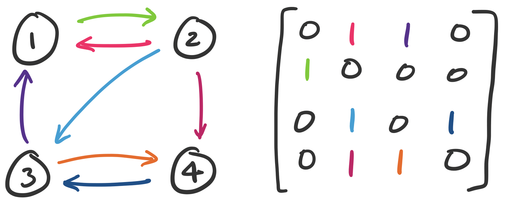
We can represent graphs as matrices by defining an adjacency matrix. Suppose each node is labelled $1$ through $n$. Then entry $a_{ij}$ is set to 1 if there is an edge $(i,j)$ in our graph and 0 otherwise.
Consider the following graph and let $A$ be its adjacency matrix. The entries of the matrix are colour-coded with the corresponding edges.
The matrix representation of a graph can be quite handy. For example, we can determine reachability by using matrix multiplication.
The number of paths from node $u$ to node $v$ is $A_{uv}^k$.
To see this, consider the following matrices for our graph above.
    >>> A = np.array([[0, 1, 1, 0], [1, 0, 0, 0], [0, 1, 0, 1], [0, 1, 1, 0]])
    >>> A @ A
    array([[1, 1, 0, 1],
           [0, 1, 1, 0],
           [1, 1, 1, 0],
           [1, 1, 0, 1]])
    >>> A @ A @ A
    array([[1, 2, 2, 0],
           [1, 1, 0, 1],
           [1, 2, 1, 1],
           [1, 2, 2, 0]])
    >>> A @ A @ A @ A
    array([[2, 3, 1, 2],
           [1, 2, 2, 0],
           [2, 3, 2, 1],
           [2, 3, 1, 2]])
A result from graph theory says that in a graph of $n$ nodes, if a node $v$ is reachable from node $u$, then there is always a path of length at most $n$. This means that we can test connectivity by considering $A^n$. Realistically, this is relatively expensive, even if we diagonalize the matrix: for a graph of $n$ nodes, our adjacency matrix is $n \times n$. If we diagonalize our matrix, we still perform at least one matrix multiplication which is at worst something like $O(n^{2.373})$ operations. Simple graph search algorithms like breadth- and depth-first search run linearly in the number of edges and nodes.
Another way to use the matrix is instead of using a binary entry (1 or 0) to denote the presence of an edge, we can instead assign it a weight. This leads us to the following example.
A (column-)stochastic matrix, also called a Markov matrix, is a matrix in which the entries of the matrices are probabilities (i.e. they are real numbers between 0 and 1) and the sum of the entries of each column is 1.
We can consider one of these matrices $A = \begin{bmatrix} \frac 1 2 & \frac 1 4 \\ \frac 1 2 & \frac 3 4 \end{bmatrix}$. This matrix can then be represented as a graph:
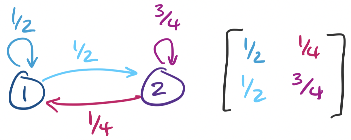
This graph represents a Markov chain. Informally, a Markov chain represents a random process that evolves probabilitically based only on the current state of the process. Each state of a Markov chain is represented by a node in our graph and the possible transitions from that state are weighted by probability.
Traditionally, the question that we want an answer for is what this system looks like as time goes on. In other words, when we take, say, 100 or 1000 or 10000 steps on this Markov chain, where do we end up? To answer this, we have to ask what $A^{10000}$ is. This is an expensive computation to do directly (especially without the help of a computer), so we diagonalize $A$. To do this, we compute the eigenvalues and eigenvectors of $A$.
    >>> A = np.array([[1/2, 1/4], [1/2, 3/4]])
    >>> L, X = np.linalg.eig(A)
    >>> L
    array([0.25, 1.  ])
    >>> X
    array([[-0.70710678, -0.4472136 ],
           [ 0.70710678, -0.89442719]])
So we can represent $A$ as $X \Lambda X^{-1}$ and therefore $A^k = X \Lambda^k X^{-1}$. The question we want to know is what happens when we take a large number of steps. In other words, what happens when $k$ gets very, very large? With a small system like this and modern computing power, we can just test this numerically:
    >>> X @ np.diag(L ** 100) @ np.linalg.inv(X)
    array([[0.33333333, 0.33333333],
           [0.66666667, 0.66666667]])
This tells us that after 100 steps, no matter where we started, we have a $\frac 1 3$ chance of being in state 1 and $\frac 2 3$ probability of being in state 2. This makes sense: while there's an equal probability of going to either state when in state 1, we have a higher chance of staying in state 2 once we've entered it.
However, in this case, diagonalization gives us a way to figure this out even without computing the power itself. The hint is in looking at what $\Lambda^k$ becomes when $k$ gets large:
    >>> L ** 100
    array([6.22301528e-61, 1.00000000e+00])
Recall that $1^k = 1$ no matter how large $k$ gets. However, $\left(\frac 1 4\right)^k = \frac{1}{4^k}$, which shrinks the larger $k$ gets. This means that we can treat it like 0. Formally, we write this kind of thing like $\Lambda^k = \begin{bmatrix} 0 & 0 \\ 0 & 1 \end{bmatrix}$ as $k \to \infty$. If we replace L ** 100 with [0, 1], we get the product
    >>> X @ np.diag([0,1]) @ np.linalg.inv(X)
    array([[0.33333333, 0.33333333],
           [0.66666667, 0.66666667]])
The most famous recent application of this idea is Google's PageRank algorithm, which was defined by Brin, Page, Motwani, and Winograd in 1998. At the time, the dominant paradigm of search was keyword-based. Search engines would try to retrieve results based on how well pages matched keywords. However, there was a problem—what separates, say, the CDC website from some guy's Geocities site (maybe the modern equivalent is some guy's Medium post)?
In other words, simply matching based on keywords is not good enough—we need a way to determine the importance or reputation of a website. This seems subjective, but it was understood to be a problem that needed solving—at the same time, there were "directories" that were keyword or topic-based lists of websites that were curated by humans.
PageRank is an algorithm that attempts to solve this "page ranking" problem (though the algorithm is really named for Larry Page). There are two pieces here to set up.
How are scores computed? The idea is based on the idea of citation counts: roughly speaking, a more important page is likely to receive more inbound links. But this assumes that every inbound link is equally important. In fact, if an inbound link comes from a highly reputable source, it should have a higher score. So an originating webpage's score contributes to the score of a page that it links to.
There is one possible pitfall here: that this score can be gamed. One immediate thing we can do is discard any self-links. Even then, one can imagine a scenario where someone tries to "trade favours" by running a large website that becomes reputable by promising links to other pages. To counter this, the amount that a page contributes to outgoing links is scaled by the total number of its outgoing links. That is, if page $i$ has score $x_i$ and has $n_i$ outgoing links, then each link provides $\frac{x_i}{n_i}$ to the receiving page. This leads us to the following setup.
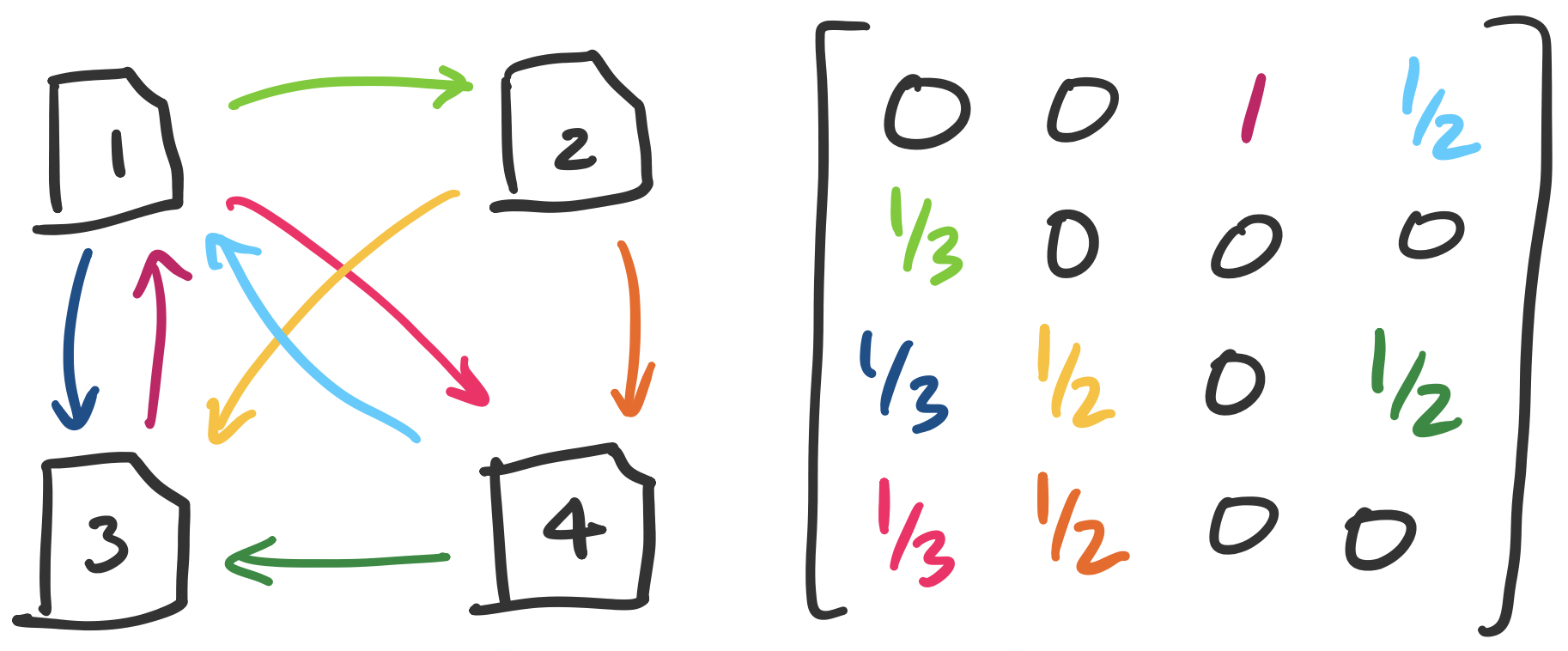
This seems to produce a bit of a chicken-and-egg scenario: in order to compute $x_1$, we need to know $x_3$ and $x_4$, but to compute both of those we would need to know $x_1$. However, what we have is really just a system of linear equations and we would like to solve for the $x_i$'s. Our example gives us the system \begin{align*} 1 x_3 + \frac 1 2 x_4 &= x_1 \\ \frac 1 3 x_1 &= x_2 \\ \frac 1 3 x_1 + \frac 1 2 x_2 +\frac 1 2 x_4 &= x_3 \\ \frac 1 3 x_1 + \frac 1 2 x_2 &= x_4 \end{align*} When viewed in matrix-vector form, we have the equation \[\begin{bmatrix} 0 & 0 & 1 & \frac 1 2 \\ \frac 1 3 & 0 & 0 & 0 \\ \frac 1 3 & \frac 1 2 & 0 & \frac 1 2 \\ \frac 1 3 & \frac 1 2 & 0 & 0 \end{bmatrix} \begin{bmatrix} x_1 \\ x_2 \\ x_3 \\ x_4 \end{bmatrix} = \begin{bmatrix} x_1 \\ x_2 \\ x_3 \\ x_4 \end{bmatrix}. \]
Disentangling this, we see that we have what amounts to an adjacency matrix weighted by the number of outgoing edges in each node. The resulting equation looks a bit strange at first:$A \mathbf x = \mathbf x$. If we squint hard enough, we notice that this is really describing an eigenvector with eigenvalue 1. The question we are then faced with is whether there exists a vector $\mathbf x^*$ such that $A \mathbf x^* = \mathbf x^*$—in other words, does $A$ have 1 as an eigenvalue?