Unfortunately, there is no built-in vector data type in Python. Some people viewed this as part of a bigger problem that needed to be fixed. The result is the Python package NumPy, which we will be using for this class.
The main contribution of NumPy is the implementation of an array class, that can be used to support vector and matrix representation.
Conceptually, a list in Python is a sequential data structure that can be extended. While Python has a particular implementation of lists, there is no guarantee that this underlying representation needs to be consistent. On the other hand, an array is a data structure that is, by definition, fixed-length and stored contiguously in memory. The second part, its representation in memory, is what allows for operations on arrays to be fast (very important in numerical computation).
One convenience of this representation is that the operations that we would like to perform on vectors essentially work the way we'd expect them to for arrays. For instance, we can perform "vector addition".
    >>> import numpy as np    # we will assume this from now on
    >>> u = np.array([3, 5])
    >>> v = np.array([7, 2])
    >>> u + v
    array([10,  7])
Note that when adding two vectors together, by definition, they need to be the same size. For instance, we cannot add the vectors $\begin{bmatrix}3 \\ 1\end{bmatrix}$ and $\begin{bmatrix}-2 \\ 4 \\ 7 \end{bmatrix}$ together.
    >>> u = np.array([3, 1])
    >>> v = np.array([-2, 4, 7])
    >>> u + v
    ValueError: operands could not be broadcast together with shapes (2,) (3,)
We can also apply "scalar multiplication" to arrays in the way we'd like to with vectors.
    >>> u = np.array([4, -2])
    >>> v = np.array([3, -1, 5])
    >>> 3 * u
    array([12, -6])
    >>> (1/4) * v
    array([ 0.75, -0.25,  1.25])
Let's think a bit about geometry, which is really about putting mathematical objects in some kind of space. Most people are first introduced to vectors in this way, usually in a physics class. Typically, we think of vectors geometrically in 2 and 3 dimensions over real scalars because that is the world that we inhabit. Doing this can be helpful for developing intiution for how vectors behave beyond two or three dimensions or things other than real numbers—you'll see a lot of people framing concepts geometrically even in higher dimensions. A lot of things in mathematics and computer science become very difficult once you go beyond three dimensions, but linear algebra happens not be one of them—a lot of ideas happen to generalize very nicely.
As we saw before, vectors are geometrically represented as arrows that are drawn from the origin, and jutting out towards a point in space specified by the components of the vector. This gives us two obvious properties of a vector: direction and length.
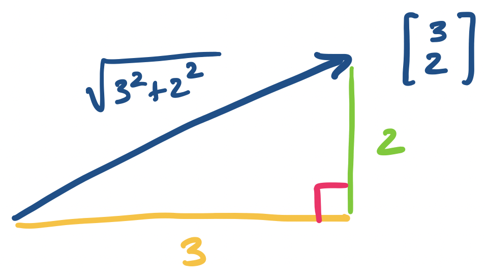
The length of a vector $\mathbf v = \begin{bmatrix} v_1 \\ v_2 \\ \vdots \\ v_n\end{bmatrix}$ is \(\|\mathbf v\| = \sqrt{v_1^2 + v_2^2 + \cdots + v_n^2}\).
Consider the vector $\mathbf v = \begin{bmatrix} 3 \\ 2 \end{bmatrix}$. By definition, its length is $\sqrt{3^2 + 2^2} = \sqrt{13}$.
The reason why this makes sense as a definition for length is pretty clear in two dimensions if you remember how triangles work. It turns out this idea carries over to higher dimensions.
This is the usual Euclidean notion of length, which is just how "far" away it is from the origin. One fun thing to do is to think about what other kinds of "length" we might be able to define on vectors and still have such a notion still make some kind of sense—the proper mathematical terminology for such functions is a norm. Here, our definition of the length of the vector is also called the Euclidean norm.
This is also referred to as the norm of a vector, for reasons that we'll eventually discuss. I mention this because this is the name of the function in NumPy.
    >>> v = np.array([3, 2])
    >>> (v[0]**2 + v[1]**2)**(1/2)   # square roots are 1/2-powers
    3.605551275463989
    >>> np.linalg.norm(v)
    3.605551275463989
The concept of the length of a vector is important because we can have multiple vectors in the same "direction" but of different lengths. In a sense, these are all the same "kind" of vector, since they can be expressed as a very simple linear combination of each other—via scalar multiplication (hence, "scalar"). This leads to the concept of a unit vector, which can be thought of as a "standard" vector for all of these vectors headed in the same direction.
A unit vector $\mathbf v$ is a vector with length $1$.
We can take any vector and find a unit vector in the same direction by "normalizing" it.
Let $\mathbf v$ be a vector. Then $\frac 1 {\|\mathbf v\|} \mathbf v$ is a unit vector in the same direction as $\mathbf v$.
Notice here that $\frac{1}{\|\mathbf v \|}$ is a scalar: the length of $\mathbf v$ is a real number and its inverse is a real number, so we're really scaling the vector. Once we know this, it becomes a bit more clear what's happening intuitively. We want a vector that's going in the same direction as $\mathbf v$, so let's scale it down by its length—this should result in a vector that has length 1.
This computation is pretty onerous to do by hand, but is pretty easily done with a computer.
    >>> v = np.array([3, 2])
    >>> 1/np.linalg.norm(v)
    0.2773500981126146
    >>> 1/np.linalg.norm(v) * v
    array([0.83205029, 0.5547002 ])
    >>> np.linalg.norm(1/np.linalg.norm(v) * v)
    1.0
Once we have the notion of length, we can also think about distances between vectors.
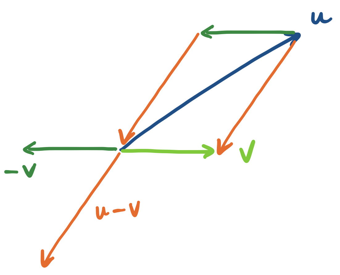
Let $\mathbf u$ and $\mathbf v$ be vectors. The distance between $\mathbf u$ and $\mathbf v$ is $\|\mathbf u - \mathbf v \|$.
It's worth thinking about what this definition is saying. First, we notice that $\mathbf u - \mathbf v$ is a vector: subtraction is just a combination of addition and scaling one vector by $-1$. So we define the distance to be the length of the vector that takes us from $\mathbf u$ to $\mathbf v$.
This is a pretty simple computation to perform.
    >>> u = np.array([-4, 1])
    >>> v = np.array([3, 2])
    >>> u-v
    array([-7, -1])
    >>> np.linalg.norm(u-v)
    7.0710678118654755
Distances are useful because in many applications, we can treat the distance as a similarity measure. Suppose a vector $\mathbf v = \begin{bmatrix} 2.3 \\ 4.22 \\ -1.7 \end{bmatrix}$ represents, say, a Spotify user and the numbers are some computed score for how much they like a particular artist or genre. If we associate each user with a vector, we can ask questions like how similar one user is to another user. One way to do this with the definitions we have so far is to compute the distance between the two vectors.
This notion of similarity is pretty straightforward and is often used in many applications. It makes sense because it's an obvious definition, but it's also easy to visualize: of course two things are more similar if they're closer together.
Now, we introduce a very useful quantity: the dot product of two vectors. This is what you would get if you were to say wait a minute—we don't really have multiplication of vectors, because scalar multiplication is just multipliying a number with a vector.
The dot product of vectors $\mathbf u = \begin{bmatrix}u_1 \\ u_2 \\ \vdots \\ u_n \end{bmatrix}$ and $\mathbf v = \begin{bmatrix} v_1 \\ v_2 \\ \vdots \\ v_n \end{bmatrix}$ is \[\mathbf u \cdot \mathbf v = u_1 v_1 + u_2 v_2 + \cdots + u_n v_n.\]
It's important here that the vectors have the same dimension (i.e. they have the same number of entries). We want the vectors to "live" in the same "space", which means, for our purposes, that they have the same number of dimensions. This notion will be formalized later on.
Let $\mathbf u = \begin{bmatrix}4 \\ 2 \\ -1\end{bmatrix}$ and $\mathbf v = \begin{bmatrix} 2 \\ -3 \\ 5 \end{bmatrix}$. Then \[\mathbf u \cdot \mathbf v = 4 \times 2 + 2 \times -3 + -1 \times 5 = -3.\]
Notice that the dot product is a scalar.
There are two main ways to apply the dot product. The first is via NumPy's dot function. The other is to use the @ operator.
    >>> u = np.array([4, 2, -1])
    >>> v = np.array([2, -3, 5])
    >>> u * v
    array([ 8, -6, -5])
    >>> np.dot(u, v)
    -3
    >>> u @ v
    -3
Something to be extremely careful of is that u * v does not give you $\mathbf u \cdot \mathbf v$. Instead, it is shorthand for "element-wise multiplication", which is the shorthand for $\begin{bmatrix} u_1 \times v_1 \\ u_2 \times v_2 \\ u_3 \times v_3 \end{bmatrix}$. This is not a linear algebra or vector operation, so you should not use it.
This is actually a good reminder that NumPy arrays are not quite vectors. They are arrays and the primary job of NumPy is to work with arrays. This means that there are operations and conveniences that are intended for usage as arrays.
One interesting observation is that the length of a vector is related to the dot product: \[\|\mathbf v\|^2 = \mathbf v \cdot \mathbf v.\] Notice that this means that a unit vector $\mathbf v$ has $\mathbf v \cdot \mathbf v = 1$.
This leads to the question of what happens when $\mathbf u \cdot \mathbf v = 0$. Of course, if $\mathbf v \cdot \mathbf v = 0$, this means that we must have $\mathbf v = 0$. But otherwise, we get the following.
For any two vectors $\mathbf u$ and $\mathbf v$, $\mathbf u \cdot \mathbf v = 0$ if and only if $\mathbf u$ is perpendicular to $\mathbf v$.
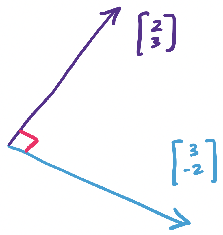
Let $\mathbf u = \begin{bmatrix} 3 \\ -2 \end{bmatrix}$. We claim that $\mathbf v = \begin{bmatrix} 2 \\ 3 \end{bmatrix}$ is perpendicular to $\mathbf u$. We can verify by this by checking their dot product:
\[\mathbf u \cdot \mathbf v = 3 \times 2 + (-2) \times 3 = 0.\]
Indeed, if we draw this out, we get:
Why does this work? When we view vectors geometrically, we can consider the "angle" that is formed between them. The dot product happens to be proportional to the cosine of this angle.
For all vectors $\mathbf u$ and $\mathbf v$, $\mathbf u \cdot \mathbf v = \|\mathbf u\| \|\mathbf v\| \cos \theta$.
We won't prove this, but this gives us an idea for why the dot product can capture a notion of similarity—but based on the direction of the vectors rather than their distance.
Recall that the cosine function takes as input some angle and produces some real number in the interval $[-1,1]$. The important points to keep in mind are:
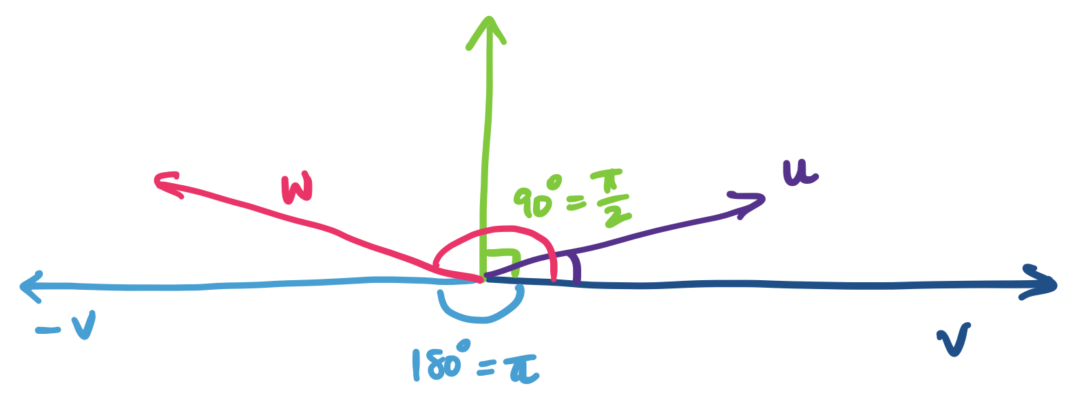
That is, the dot product can capture how similar two vectors are in terms of their direction. If the two vectors are pointing in roughly the same direction, their dot product will be positive; otherwise if they're pointing away from each other, it'll be negative. Notice that the closer they are to either the original direction or its opposite, the "intensity" of $\cos \theta$ increases. If the vectors are completely orthogonal, then we get 0.
In the above diagram, $\mathbf u \cdot \mathbf v$ is positive, since its angle is between 0 and 90 degrees, while $\mathbf v \cdot \mathbf w$ is negative, since its angle is between 90 and 180 degrees. If $\mathbf u$ is closer to $\mathbf v$, the cosine of the angle is closer to 1 and if it is closer to the green vector, the cosine of the angle gets closer to 0. Similarly, if $\mathbf w$ is closer to $\mathbf -v$, the cosine of the angle it makes with $\mathbf v$ gets closer to $-1$, while the closer it is to the green vector, the closer the cosine of its angle gets to 0, but on the negative side.
This makes sense for a two-dimensional vector but this property still holds in higher dimensions. The reason for this is pretty simple: if I have two vectors in any number of dimensions, I can always find a plane that they lie on and figure out an angle between them.
What can the dot product tell us? Suppose again that our vectors represent, say, a Spotify user's tastes in various genres of music. We've already seen that we can compare two users' tastes by considering the distance between their "taste vectors". But here's something we can do with the dot product.
Suppose that we would like to identify certain users with certain mixes of tastes. Let's say that a vector $\begin{bmatrix} v_1 \\ v_2 \\ v_3 \end{bmatrix}$ represents a user's preference or not for rock, ska, and Eurobeat, respectively. We can design a "template" user that prefers rock, detests ska, and is indifferent to Eurobeat by the vector $\begin{bmatrix} 100 \\ -100 \\ 0 \end{bmatrix}$. Then taking the dot product of a vector with this template, $100v_1 - 100v_2 + 0v_3$, will give us a scalar quantity. The larger that quantity is, the more similar the user is to our template, and the smaller (i.e. negative) it is, the less similar they are. In some sense, our template "weights" the genre scores.
It's maybe a bit early for this and we don't really get into it much, but it's interesting to note that these are not arbitrary definitions. Instead, they are consequences of the idea that vectors are things that we can add and scale. If we used weirder scalars, we would be able to come up with similarly appropriate definitions. (These more general dot products have a name—they're called inner products and the dot product is a specific instance of an inner product)