What we've accomplished so far works for projections onto subspaces. That is, if all we want to do was take a subspace and we know its basis, we can transform that basis into an orthogonal basis and then go to town with the result. However, things get trickier when we want to solve or approximate a specific linear equation $A \mathbf x = \mathbf b$—we can't just transform $A$ into $Q$ and call it a day.
We have to remember that, as with any transformation to our matrix $A$ that we make, whether it is the row-reduced echelon form $R$ or the upper triangular matrix $U$, transforming $A$ means that there will be another matrix involved that contains the information that we "lose" when transforming from $A$ to our new form
For the row-reduced echelon form $R$, this is the matrix $C$ containing independent columns, to get us $A = CR$. For the upper-triangular matrix $U$, this is the matrix $L$ containing the elimination constants, to get us $A = LU$. For the orthogonal matrix $Q$, this matrix is called $R$ (confusingly, not the same $R$ that we've been using), which gives us $A = QR$.
The QR factorization of an $m \times n$ matrix $A$ is given by $A = QR$, where $Q$ is an orthogonal matrix and $R$ is an upper triangular matrix, defined by \[A = \begin{bmatrix} \\ \mathbf a_1 & \mathbf a_2 & \cdots & \mathbf a_n \\ \\ \end{bmatrix} = \begin{bmatrix} \\ \mathbf q_1 & \mathbf q_2 & \cdots & \mathbf q_n \\ \\ \end{bmatrix} \begin{bmatrix} \mathbf q_1^T \mathbf a_1 & \mathbf q_1^T \mathbf a_2 & \mathbf q_1^T \mathbf a_3 & \cdots & \mathbf q_n^T \mathbf a_n \\ 0 & \mathbf q_2^T \mathbf a_2 & \mathbf q_2^T \mathbf a_3 & \cdots & \mathbf q_2^T \mathbf a_n \\ 0 & 0 & \mathbf q_3^T \mathbf a_3 & \cdots & \mathbf q_3^T \mathbf a_n \\ \vdots & \vdots & & \ddots & \vdots \\ 0 & 0 & \cdots & 0 & \mathbf q_n^T \mathbf a_n \end{bmatrix} = QR.\]
It is clear that $Q$ contains the orthonormal basis of the column space spanned by columns of $A$. But what about $R$? If we examine closely, we see that each entry of the matrix $R$ is defined as follows, \[r_{ij} = \begin{cases} \mathbf q_i^T \mathbf a_j & \text{if $i \leq j$,} \\ 0 & \text{otherwise.} \end{cases}\]
The result is that $\mathbf a_i$ can be written as a linear combination of $\mathbf q_i$'s. The matrix $R$ tells us exactly how: \[\mathbf a_i = \mathbf q_1 (\mathbf q_1^T \mathbf a_i) + \cdots + \mathbf q_i (\mathbf q_i^T \mathbf a_i).\]
What does this mean? Since $\mathbf q_1, \dots, \mathbf q_n$ is an orthonormal basis for the column space of $A$, this is describing each column $\mathbf a_i$ in terms of the $\mathbf q$ basis, particularly when we read the term written as $\mathbf q_i(\mathbf q_i^T \mathbf a_j$) with $\mathbf q_i^T \mathbf a_j$ acting as the scaling factor. But if we shift the parentheses and read the term as $(\mathbf q_i \mathbf q_i^T)\mathbf a_j$, we see that each term is describing a projection of $\mathbf a_j$ onto the line with basis $\mathbf q_i$. This makes sense, since what we did to each column of $A$ was split it up into its orthogonal parts.
This is a nice decomposition for a few reasons:
Let's return to $A = \begin{bmatrix}-1 & -1 & 0\\-1 & 0 & 1\\0 & -2 & -1\end{bmatrix}$. We got $Q = \begin{bmatrix}- \frac{\sqrt{2}}{2} & - \frac{\sqrt{2}}{6} & - \frac{2}{3}\\- \frac{\sqrt{2}}{2} & \frac{\sqrt{2}}{6} & \frac{2}{3}\\0 & - \frac{2 \sqrt{2}}{3} & \frac{1}{3}\end{bmatrix}$ from the Gram–Schmidt process. But what is the associated $R$? We simply go through each entry and take the appropriate dot products.
Computationally, this is not so bad. Since $A = QR$, we want to solve for $R$, which involves isolating. Since $Q$ is orthogonal, it is very easy to get rid of, by multiplying $Q^T$ in front. Do that on both sides to get \[Q^T A = Q^T (Q R) = R.\]
    >>> A = np.array([[-1, -1, 0], [-1, 0, 1], [0, -2, -1]])
    >>> Q
    array([[-0.70710678, -0.23570226, -0.66666667],
           [-0.70710678,  0.23570226,  0.66666667],
           [ 0.        , -0.94280904,  0.33333333]])
    >>> Q.T @ A
    array([[ 1.41421356e+00,  7.07106780e-01, -7.07106780e-01],
           [ 0.00000000e+00,  2.12132034e+00,  1.17851130e+00],
           [ 0.00000000e+00,  1.00000001e-08,  3.33333340e-01]])
This gives us $R = \begin{bmatrix}\sqrt{2} & \frac{\sqrt{2}}{2} & - \frac{\sqrt{2}}{2}\\0 & \frac{3 \sqrt{2}}{2} & \frac{5 \sqrt{2}}{6}\\0 & 0 & \frac{1}{3}\end{bmatrix}$.
We saw that using $Q$ improved our least squares computation, but we don't always have a perfectly orthonormal basis $Q$. We do always have $A = QR$, though. The question is whether $A = QR$ improves the situation at all. First, let's consider $A^TA$: \[A^TA = (QR)^T QR = R^TQ^TQR = R^TR.\] If we substitute this into our least squares equation, we get \begin{align*} R^TR\mathbf{\hat x} &= R^TQ^T\mathbf b \\ R\mathbf{\hat x} &= Q^T\mathbf b \end{align*} At this point, it looks like we haven't gained anything—we still need to move $R$ to the other side, so we compute $R^{-1}$. However, that omits a very crucial property of $R$. First, remember that we can compute $Q^T \mathbf b = \mathbf d$, so let's rewrite our equation: \[R \mathbf{\hat x} = \mathbf d.\] We are back to solving a linear equation. But recall that $R$ is upper triangular! This means that we can just use substitution to solve this equation and avoid the expensive computation for the inverse.
As mentioned earlier, we are now going to demand more and more of the bases for our subspaces. As a recap, we began with sets of vectors and asking about their linear combinations. Then we imposed the condition of independence on them, which gave us several useful ideas, like basis and dimension. Then we added the condition that the basis are orthonormal, which gives us convenient bases to work with conceptually and computationally.
The final missing piece is to be able to derive meaning from a basis. In other words, we would like the basis of our subspaces to have some notion of importance. This seems like a strange ask of vectors and matrices since they appear to be arbitrary collections of numbers. However, we have to remember that the whole idea of linear algebra in data science is that these collections have some latent linear substructure to them.
It turns out that this question of which "directions" of the subspace are "important" is not a totally crazy thing to ask for. These are captured by what are called eigenvectors. To understand how eigenvectors describe notions of importance in terms of direction, we have to first revisit the idea of matrices as describing linear transformations.
In order to talk about eigenvectors, we need to talk about linear transformations, and in order to talk about linear transformations, we should start with the simplest cases, where our matrices are $n \times n$—that is, transformations of vectors in the same vector space $\mathbb R^n$. As we mentioned before, it's unlikely that we'll encounter data matrices that are square. However, they still play an important role in representing certain kinds of data (for example, graphs) and are particularly important from the point of view as transformations.
First, let's look at transformations on their own.
A linear transformation $T : \mathbf U \to \mathbf V$ is a function that takes a vector in vector space $\mathbf U$ and produces a vector in vector space $\mathbf V$ such that for all vectors $\mathbf u$ and $\mathbf v$,
Notice that this definition doesn't involve matrices yet—though, obviously, like everything else in the course, it will. But the plainest reading of this definition is that it is a definition about functions, not matrices.
Here's an example that doesn't involve vectors at all: expectation of random variables. Recall that the expectation of a random variable $X$ can be thought of as the average of $X$ weighted by probabilities. It turns out that there is a theorem called "linearity of expectation" which says that $E(c_1X_1 + c_2 X_2) = c_1 E(X_1) + c_2 E(X_2)$.
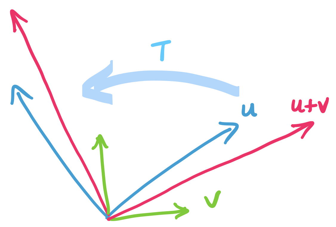
Let $T$ be a transformation that rotates a vector clockwise by $\theta$. We can test the two properties of linear transformations: If we add and scale the input then rotate it, do we end up with the same vector as if we rotated the inputs, then combined them? The answer turns out to be yes:
One of the consequences (conveniences) of the definition for linear transformations is that if we know that $\mathbf u = a_1 \mathbf v_1 + \cdots + a_n \mathbf v_n$, then it must be the case that $T(\mathbf u) = a_1 T(\mathbf v_1) + \cdots + a_n T(\mathbf v_n)$. This is important, because what it says is that in order to compute a transformation, all we really need to know is how the transformation affects the basis.
Here is a transformation that seems linear, but isn't. Recall that to darken an RGB colour by a factor of $0 \leq k \leq 1$, we define the transformation $\begin{bmatrix} r \\ g \\ b \end{bmatrix} \mapsto (1-k) \begin{bmatrix} r \\ g \\ b \end{bmatrix}$. This is linear. We can define lightening similarly: \[\begin{bmatrix} r \\ g \\ b \end{bmatrix} \mapsto \begin{bmatrix} (1-k)r + k \\ (1-k)g + k \\ (1-k)b + k \end{bmatrix}.\] However, this transformation is not linear. To see why, take two colours $(r_1, g_1, b_1)$ and $(r_2, g_2, b_2)$. If we add the two colours first, we get \[ T\left(\begin{bmatrix}r_1\\ g_1\\ b_1\end{bmatrix} + \begin{bmatrix}r_2\\ g_2\\ b_2\end{bmatrix}\right) = T\left(\begin{bmatrix}r_1 + r_2\\ g_1 + g_2\\ b_1 + b_2\end{bmatrix}\right) = \begin{bmatrix}(1-k)(r_1 + r_2)+k\\ (1-k)(g_1 + g_2)+k\\ (1-k)(b_1 + b_2)+k\end{bmatrix} \] But if we transform the colours first and then add them, this gives us \begin{align*} T\left(\begin{bmatrix}r_1\\ g_1\\ b_1\end{bmatrix}\right) + T\left(\begin{bmatrix}r_2\\ g_2\\ b_2\end{bmatrix}\right) &= \begin{bmatrix}(1-k)r_1+k\\ (1-k)g_1+k\\ (1-k)b_1+k\end{bmatrix} + \begin{bmatrix}(1-k)r_2+k\\ (1-k)g_2+k\\ (1-k)b_2+k\end{bmatrix} \\ &= \begin{bmatrix}(1-k)(r_1 + r_2)+2k\\ (1-k)(g_1 + g_2)+2k\\ (1-k)(b_1 + b_2)+2k\end{bmatrix} \end{align*} which is not the same. These are an example of affine transformations, which have the form $a T(\mathbf v) + b$.
We want to come up with a matrix that describes our rotation in $\mathbb R^2$ by some angle $\theta$. We know from geometry that rotating $\begin{bmatrix} 1 \\ 0 \end{bmatrix}$ by $\theta$ results in a vector $\begin{bmatrix} \cos \theta \\ \sin \theta \end{bmatrix}$ and rotating $\begin{bmatrix} 0 \\ 1 \end{bmatrix}$ by $\theta$ results in a vector $\begin{bmatrix} -\sin \theta \\ \cos \theta \end{bmatrix}$.
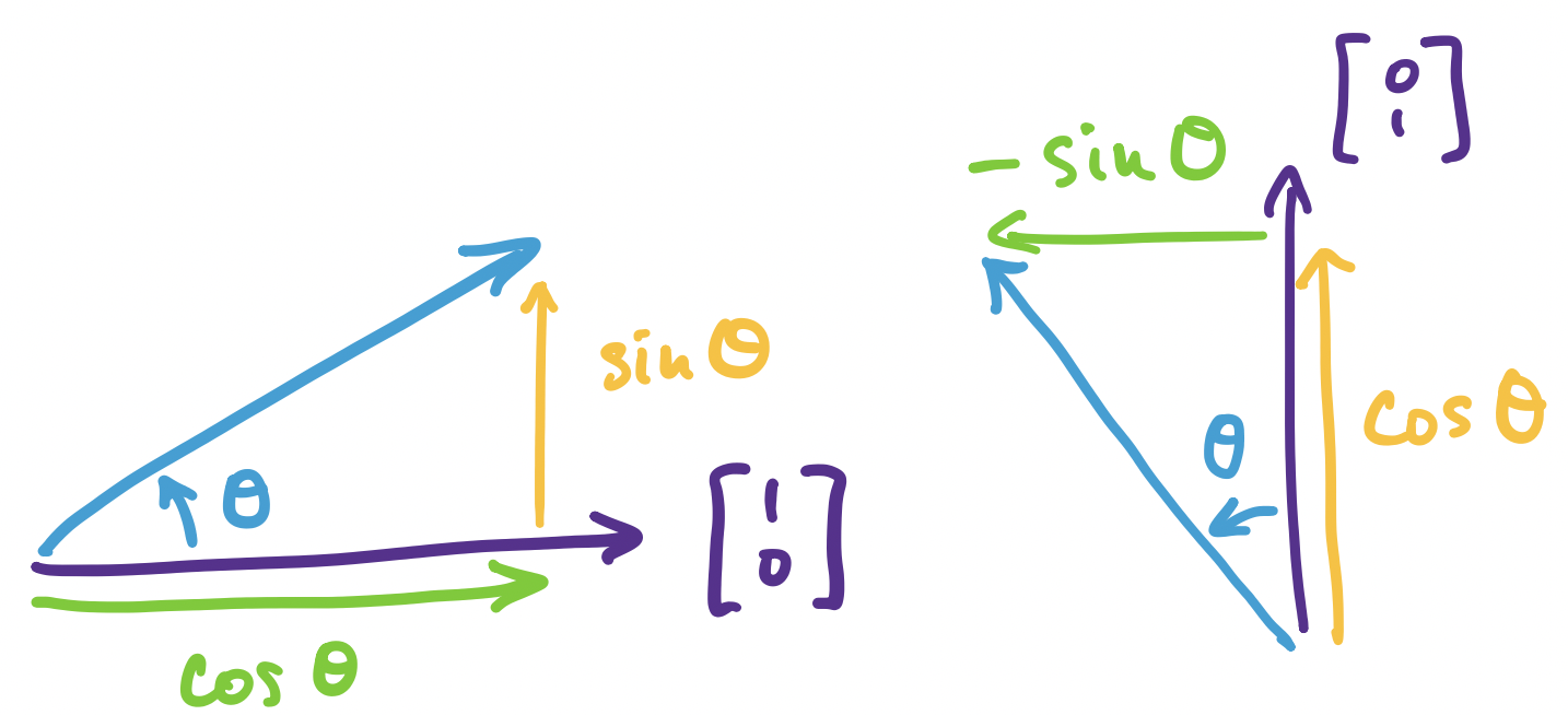
What if we have an arbitrary vector $\mathbf v = \begin{bmatrix}v_1 \\ v_2 \end{bmatrix}$? We know we can write this vector in terms of the standard basis as \(\mathbf v = v_1 \begin{bmatrix} 1 \\ 0 \end{bmatrix} + v_2 \begin{bmatrix} 0 \\ 1 \end{bmatrix}\). Then our rules about linear transformations say that the rotation of $\mathbf v$ can be described as \[v_1 \begin{bmatrix} \cos \theta \\ \sin \theta \end{bmatrix} + v_2 \begin{bmatrix} -\sin \theta \\ \cos \theta \end{bmatrix} = \begin{bmatrix} \cos \theta & - \sin \theta \\ \sin \theta & \cos \theta \end{bmatrix} \begin{bmatrix} v_1 \\ v_2 \end{bmatrix}.\]
    >>> t = np.radians(45)  # 45 degrees
    >>> A = np.array([[np.cos(t), -np.sin(t)], [np.sin(t), np.cos(t)]])
    >>> A
    array([[ 0.70710678, -0.70710678],
           [ 0.70710678,  0.70710678]])
    >>> v = np.array([2, 3])
    >>> A @ v
    array([-0.70710678,  3.53553391])
So we've recovered a matrix that describes our transformation. We can play the same trick to arrive at the fact that every linear transformation can be described via a matrix. And since every matrix is a linear transformation, by virtue of matrix multiplication obeying the rules of linear transformations, we can say that the two things are basically the same thing.
Notice that every matrix ends up defining some linear transformation, even those that are not square. These ones take a vector from $\mathbb R^m$ as input and produce a vector in $\mathbb R^n$. But first, we'll focus on $n \times n$ matrices and then see how to generalize to $m \times n$ matrices.
In the case of a square matrix, we are taking a vector in $\mathbb R^n$ and mapping it to some other vector in $\mathbb R^n$. This amounts to moving it around, squishing and stretching it into some other vector in the same space. Intuitively, this tells us that there must be some vectors that stay roughly the same under such transformations—these vectors are the eigenvectors of the matrix.
What do eigenvectors tell us? Consider some data set that looks like the following.
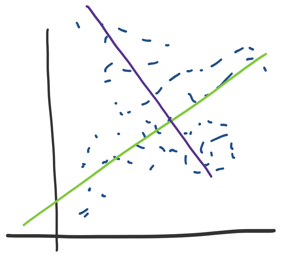
We see this kind of thing and think that we would really like to draw a line of best fit through it. Luckily, we've seen how to do exactly that. But this assumes that we've organized our data enough to know that we want to compute a regression on a specific variable. What happens if we don't know this? Perhaps we have several dimensions and we need to find one such axis or direction.
If we think of our data from the point of view of transformation, we can see that what we're trying to do is predict where to map data based on our data set—in the language of machine learning, this transformation is really the function that we're trying to "learn". One way to think about this visually is that it means that there will be some "directions" in which we send certain vectors that are more likely or that are a heavier influence. These are the directions or vectors that we are trying to find.
Intuitively, we expect that these are associated with vectors that are "stable" or don't change direction when we apply our transformation. These are exactly the eigenvectors of the matrix.
Let $A$ be an $n \times n$ matrix. A scalar $\lambda$ is an eigenvalue of $A$ if $A \mathbf x = \lambda \mathbf x$ for some vector $\mathbf x$. The vector $\mathbf x$ is the eigenvector that corresponds to $\lambda$.
This definition tells us that eigenvectors are those vectors that stay the same, but are scaled by a transformation—in other words, the direction of the vector doesn't change. In some sense, we can think of these vectors as remaining stable under the transformation. This suggests that they capture some information about the structure of the transformation.
Let $A = \begin{bmatrix} 7 & -9 \\ 2 & -2 \end{bmatrix}$. The vector $\begin{bmatrix} 3 \\ 1 \end{bmatrix}$ is an eigenvector of $A$. Its associated eigenvalue is 4. To see this, we have: \[\begin{bmatrix} 7 & -9 \\ 2 & -2 \end{bmatrix} \begin{bmatrix} 3 \\ 1 \end{bmatrix} = \begin{bmatrix} 12 \\ 4 \end{bmatrix} = 4 \begin{bmatrix} 3 \\ 1 \end{bmatrix}.\]
The main question we have at this point is how to find the eigenvalues and eigenvectors of a matrix.