While we've oriented our subspaces, we've said nothing about their bases—only that these exist. But because bases are how we describe our subspaces, it stands to reason that our choice of basis matters. Bases over $\mathbb R^n$ are a good example: we would rather work with the standard basis than a basis of arbitrary vectors.
In this view, the right choice of basis can make the difference between an easy and an expensive computation. Right now, the biggest challenge in computing projections and least squares solutions is the computation of inverses. As mentioned earlier, computing the inverse is an expensive operation that we always try to avoid—this is the reason why we preferred methods like LU factorization for solving linear equations.
One reason for why the standard basis is convenient is because the vectors are orthogonal. The other reason is that they are unit vectors—they have length 1. This leads us to the following definition.
A set of vectors $\mathbf q_1, \dots, \mathbf q_n$ is orthogonal when $\mathbf q_i \cdot \mathbf q_j = 0$ for all $i \neq j$. They are orthonormal if \[\mathbf q_i \cdot \mathbf q_j = \begin{cases} 0, & \text{if $i \neq j$, and } & \text{(orthogonal)} \\ 1, & \text{if $i = j$}. & \text{(unit vectors)} \end{cases}\] Notice that, by convention, we use $\mathbf q$ to denote orthonormal vectors.
There are two very useful observations to make here. One is that orthonormal vectors will "cancel" each other out to become zero. The other is that the same vectors will remain constant because they "combine" to make 1. This seems like a path forward to simplifying computations. Indeed, we immediately get the following.
Let $Q$ be an $m \times n$ matrix wtih orthonormal columns. Then $Q^TQ = I$. Furthermore, if $m = n$ (so $Q$ is square), $Q^T = Q^{-1}$.
To see this, consider each entry $q_{ij}$ of the matrix $Q^T Q$. The entry $q_{ij}$ is exactly the product $\mathbf q_i^T \mathbf q_j$. Since these vectors are all orthonormal, we have that \[q_{ij} = \begin{cases} 0 & \text{if $i \neq j$}, \\ 1 & \text{if $i = j$.} \end{cases}\] This means that the off-diagonal entries are all 0 and the diagonal entries are all 1. This is exactly $I$.
The nice properties of orthonormal vectors suggest that they would make for an ideal basis for any subspace. For instance, consider the problem of computing least squares approximations: \begin{align*} Q^TQ \mathbf{\hat x} &= Q^T \mathbf b \\ \mathbf{\hat x} &= Q^T \mathbf b & \text{since $Q^TQ = I$} \end{align*} Notice that since $Q^TQ$ disappears, we have no need to compute the inverse anymore to get $\mathbf{\hat x}$. From here, we get \[\mathbf p = Q \mathbf{\hat x} = QQ^T \mathbf b = \mathbf q_1 (\mathbf q_1^T \mathbf b) + \cdots + \mathbf q_n (\mathbf q_n^T \mathbf b).\] This makes sense: if we consider any one of the projections, we would have $\mathbf q_i \left( \frac{\mathbf q_i^T \mathbf b}{\mathbf q_i^T \mathbf q_i}\right)$ by definition. But since $\|\mathbf q_i\| = 1$, we have $\mathbf q_i^T \mathbf q_i = \|\mathbf q_i\|^2 = 1$ so the denominator gets simplified away. This also tells us that the projection matrix is: \[P = Q(Q^TQ)^{-1}Q^T = QQ^T,\] which sees the projection matrix as a sum of the projection matrices for each column.
Like vectors, we denote matrices with orthonormal columns by $Q$. Note that $Q$ is not necessarily square. Square matrices that have orthonormal columns are, somewhat confusingly, called orthogonal matrices.
Consider the matrix $A = \begin{bmatrix}-1 & -1 & 0\\-1 & 0 & 1\\0 & -2 & -1\end{bmatrix}$. The columns of $A$ are independent, but not orthogonal. The following matrix has orthonormal columns. \[\begin{bmatrix}- \frac{\sqrt{2}}{2} & - \frac{\sqrt{2}}{6} & - \frac{2}{3}\\- \frac{\sqrt{2}}{2} & \frac{\sqrt{2}}{6} & \frac{2}{3}\\0 & - \frac{2 \sqrt{2}}{3} & \frac{1}{3}\end{bmatrix}\]
One challenge we will face computationally is that we need to use floating point representations of these numbers.
We've already seen an example of an orthogonal matrix—every permutation matrix is orthogonal! \[\begin{bmatrix} 0 & 0 & 1 & 0 & 0\\ 0 & 0 & 0 & 0 & 1\\ 0 & 0 & 0 & 1 & 0\\ 0 & 1 & 0 & 0 & 0\\ 1 & 0 & 0 & 0 & 0 \end{bmatrix}\] It's not hard to see that all the columns of any permutation matrix are orthonormal. We have also already seen that its inverse is exactly its transpose.
It is all well and good that orthonormal bases exist, but how do we find them? Luckily, there's at least one simple algorithm that shows us this can be done.
For any set of basis vectors $\mathbf a_1, \dots, \mathbf a_n$, we can construct an orthogonal basis $\mathbf b_1, \dots, \mathbf b_n$ for the same vector space, defined by
This algorithm is called the Gram–Schmidt process.
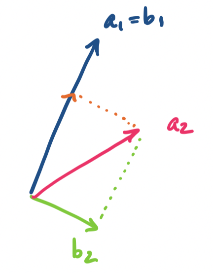
Suppose we have three vectors. Then the first vector we choose is our starting point $\mathbf b_1 = \mathbf a_1$. We take the next vector, $\mathbf a_2$ and subtract its projection onto $\mathbf b_1$ from it to get $\mathbf b_2$. This looks like the following:
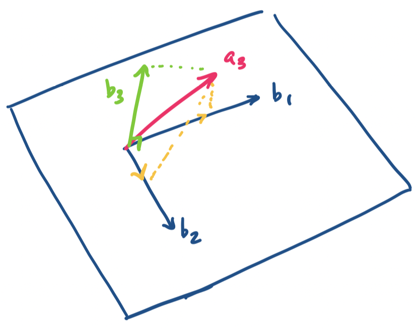
Then we repeat that process: take $\mathbf a_3$ and subtract its projections on $\mathbf b_1$ and $\mathbf b_2$. We are left with a vector that is orthogonal to both:
In other words, we construct each orthogonal basis vector in sequence. For each new vector $\mathbf a_i$ we want to add to our basis, we subtract from it the projections of the orthogonal vectors $\mathbf b_j$ we've constructed so far.
Alternatively, we can think of it as doing the following: we project the vector onto the subspace of orthogonal vectors we've found so far and take the error vector, which is orthogonal to the projection. The new vector is then guaranteed to be orthogonal to those vectors and we add it to the basis and repeat the process..
Note that these vectors are not yet orthonormal. All we've done is construct a set of orthogonal vectors. Technically speaking, the Gram–Schmidt process only deals with the problem of finding a set of orthogonal vectors. However, normalizing them is simple: for each $\mathbf b_i$, take $\mathbf q_i = \frac 1 {\|\mathbf b_i\|} \mathbf b_i$. Whether you choose to normalize them all at once or as you go along is up to you to decide.
Let $A = \begin{bmatrix}-1 & -1 & 0\\-1 & 0 & 1\\0 & -2 & -1\end{bmatrix}$. We want to compute an orthonormal basis for the column space of $A$.
We will be doing this entirely computationally, so we will not bother with tracing out the calculations. We will also be normalizing each result as we go along.
First, we simply take $\mathbf b_1 = \frac{\mathbf a_1}{\|\mathbf a_1\|}$.
    >>> A = np.array([[-1, -1, 0], [-1, 0, 1], [0, -2, -1]])
    >>> b1 = A[:,[0]] / np.linalg.norm(A[:,[0]])
    >>> b1
    array([[-0.70710678],
           [-0.70710678],
           [ 0.        ]])
For the next vector $\mathbf a_2 = \begin{bmatrix} -1 \\ 0 \\ -2 \end{bmatrix}$, we need to project it onto $\mathbf b_1$ and subtract that piece from it. This is the expression \[\mathbf b_2' = \mathbf a_2 - \mathbf b_1 \frac{\mathbf b_1^T \mathbf a_2}{\mathbf b_1^T \mathbf b_1} = \mathbf a_2 - \mathbf b_1 \mathbf b_1^T \mathbf a_2.\] Notice that the denominator goes away because we normalized $\mathbf b_1$. Once we get $\mathbf b_2'$ we normalize it to get $\mathbf b_2 = \frac{\mathbf b_2'}{\|\mathbf b_2'\|}$.
    >>> b2 = A[:,[1]] - b1 * b1.T @ A[:,[1]]
    >>> b2 = b2/np.linalg.norm(b2)
    >>> b2
    array([[-0.23570226],
           [ 0.23570226],
           [-0.94280904]])
For the final vector $\mathbf a_3 = \begin{bmatrix} 0 \\ 1 \\ -1 \end{bmatrix}$, we do the same thing but we have two other orthogonal vectors to deal with. We subtract $\mathbf a_3$ from projections on $\mathbf b_1$ and $\mathbf b_2$. Recalling that $\mathbf b_1$ and $\mathbf b_2$ are unit vectors, we obtain \[\mathbf b_3' = \mathbf a_3 - \mathbf b_1 \mathbf b_1^T \mathbf a_3 - \mathbf b_2 \mathbf b_2^T \mathbf a_3,\] which we need to normalize to arrive at $\mathbf b_3$.
    >>> b3 = A[:,[2]] - b1 * b1.T @ A[:,[2]] - b2 * b2.T @ A[:,[2]]
    >>> b3 = b3/np.linalg.norm(b3)
    >>> b3
    array([[-0.66666667],
           [ 0.66666667],
           [ 0.33333333]])
Finally, we take our computed vectors and put them together into a single matrix $Q$.
    >>> Q = np.hstack((b1, b2, b3))
    >>> Q
    array([[-0.70710678, -0.23570226, -0.66666667],
           [-0.70710678,  0.23570226,  0.66666667],
           [ 0.        , -0.94280904,  0.33333333]])
Doing this exactly would have yielded the matrix $Q = \begin{bmatrix}- \frac{\sqrt{2}}{2} & - \frac{\sqrt{2}}{6} & - \frac{2}{3}\\- \frac{\sqrt{2}}{2} & \frac{\sqrt{2}}{6} & \frac{2}{3}\\0 & - \frac{2 \sqrt{2}}{3} & \frac{1}{3}\end{bmatrix}$.
    >>> np.array([[-2**0.5 / 2, -2**0.5 / 6,    -2/3],
    ...           [-2**0.5 / 2,  2**0.5 / 6,     2/3],
    ...           [0,           -2 * 2**0.5 / 3, 1/3]])
    array([[-0.70710678, -0.23570226, -0.66666667],
           [-0.70710678,  0.23570226,  0.66666667],
           [ 0.        , -0.94280904,  0.33333333]])
One way to think about this is to treat this as "building" the basis for our subspace iteratively, adding a dimension on each step. We begin with one vector. We take the next vector and consider the subspace defined by that vector and everything orthogonal to it. We know that we can split our vector up into a projection onto the first vector and something orthogonal to it. Now, we have two orthogonal vectors that can be combined into our original second vector.
On each subsequent step, we keep splitting our successive basis vectors into a part that projects onto a subspace of dimension $k-1$ and something orthogonal to that, which we take as our $k$th basis vector, until we have our desired basis.