Projections lead us a tool that answers the question of what to do when we are faced with a linear equation $A \mathbf x = \mathbf b$ with no solution. Recall that in such cases, we have a vector that lines outside of the column space of $A$. In other words, we have a sample that lies outside of our model for our dataset. This is not an uncommon situation so we can't just throw up our hands and give up. So, what to do?
Our discussion of projections has already hinted at this: find the closest point that is in the desired subspace. What this means is that for a matrix $A$, if $\mathbf b$ is not in the column space of $A$, we want to find instead a solution for the vector in the column space of $A$ that is closest to $\mathbf b$. We already have an answer for this: it's the projection of $\mathbf b$ onto the column space of $A$!
The key here is something we mentioned offhandedly earlier: that the projection is the vector in the column space of $A$ for which the error is minimized. Here, the error is the vector $\mathbf e = \mathbf b - \mathbf p$ and the length of that error is $\|\mathbf e\|$.
Recall that by definition, we have $\mathbf p = A \mathbf{\hat x}$, so we have $\mathbf e = \mathbf b - A \mathbf{\hat x}$. By this, we have that $\|\mathbf e\| = \|\mathbf b - A \mathbf{\hat x}\|$. To minimize $\|\mathbf e\|$, we need to minimize $\|\mathbf b - A \mathbf{\hat x}\|^2$, which leads us to what you may know as the least squares approximation.
First, let's consider this problem geometrically. Consider the three points $(0,3), (1,1), (2,5)$. We want to fit a line through these points, but no single line will contain all three. Instead, we will try to find the line that will minimize the distance to all three.
Let's consider a line $b = x_0 + x_1t$. What we have with our example is trying to solve the system of equations \begin{align*} x_0 + x_1 \cdot 0 &= 3 \\ x_0 + x_1 \cdot 1 &= 1 \\ x_0 + x_1 \cdot 2 &= 5 \end{align*} This gives us matrices and vectors $A = \begin{bmatrix} 1 & 0 \\ 1 & 1 \\ 1 & 2 \end{bmatrix}$, $\mathbf b = \begin{bmatrix} 3 \\ 1 \\ 5 \end{bmatrix}$, and $\mathbf x = \begin{bmatrix} x_0 \\ x_1 \end{bmatrix}$.
Again, we realize that $\mathbf b$ lies outside of the column space of $A$. This means that there is no solution $x_0$ and $x_1$ for our line. So we must instead find $x_0$ and $x_1$ for the closest vector that is in the column space. This is our projection, and this makes the question of finding an appropriate $\begin{bmatrix} x_0 \\ x_1 \end{bmatrix}$ the same question as finding $\mathbf{\hat x}$.
Since we've already done this exact example last class in the context of projections, we have that $x_0 = 2$ and $x_1 = 1$. This gives us the line $2 + t$, which looks like it does a pretty good job of getting close to all of our points.
    >>> b = np.array([3, 1, 5])
    >>> t = np.arange(3)
    >>> A = np.ones((3,2))
    >>> A[:,1] = t
    >>> x = np.linalg.solve(A.T @ A, A.T @ b)
    >>> x
    array([2., 1.])
    >>> for i,y in enumerate(b):
    ...     plt.plot([i,i], [x[0]+x[1]*t[i], y], 'r')
    >>> plt.plot(t, b, 'o')
    >>> plt.plot(t, x[0] + x[1] * t)
    >>> plt.plot(t, A @ x, 'x')
    >>> plt.grid()
    >>> plt.show()
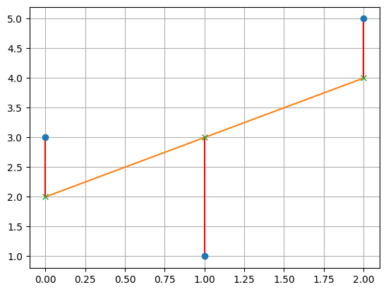
This gives us the geometric view, but how does this fit in with the vector space view? what we've shown is that $\mathbf{\hat x} = \begin{bmatrix} 2 \\ 1 \end{bmatrix}$. this means that we can compute the projection $\mathbf p$: \[\mathbf p = A \mathbf{\hat x} = 2 \begin{bmatrix} 1 \\ 1 \\ 1 \end{bmatrix} + 1 \begin{bmatrix} 0 \\ 1 \\ 2 \end{bmatrix} = \begin{bmatrix} 2 \\ 3 \\ 4 \end{bmatrix},\] which is what we got when we went through this example before. Now, if we look at the line we just drew, we notice that this is exactly the $b$ at each point on the line.
Next, we recall that the error is $\mathbf e = \mathbf b - \mathbf p$. In other words, this should be the difference between the points along the $b$-axis. If we examine the diagram, we see that this distance is 1, -2, and 1. Indeed, we have \[\mathbf e = \mathbf b - \mathbf p = \begin{bmatrix} 3 \\ 1 \\ 5 \end{bmatrix} - \begin{bmatrix} 2 \\ 3 \\ 4 \end{bmatrix} = \begin{bmatrix} 1 \\ -2 \\ 1 \end{bmatrix}.\]
How does this translate to vector spaces? Here, we have $A$, which is our model. If it's an $m \times n$ matrix, this means that we have a linear function of $n-1$ variables and $m$ points to fit. For instance, in our case $n = 2$ and we are trying to describe a function $y = x_0 + x_1t$, where $t$ is our single variable.
What transformation does $A$ make? It transforms vectors of parameters/coefficients into vectors of the "$y$" variable. Since $A$ is our model, each column is a vector of some variable (except for the first) and we are trying to combine these to get to a vector of $y$-values. Ideally, we can do this—$\mathbf b$ is in the column space. If it's not in the column space, we have to get as close as possible, by minimizing the difference at each point. This difference is captured by $\mathbf e$.
In other words, the goal is to find the parameters $\mathbf{\hat x}$ that minimizes $\mathbf e$.
The least squares solution for an equation $A \mathbf x = \mathbf b$ is $\mathbf{\hat x}$. That is, $\|\mathbf b - A\mathbf x\|^2$ is minimized when $\mathbf x = \mathbf{\hat x}$.
Recall that for any vector $\mathbf b$ in $\mathbb R^m$, it can be written as two vectors: one in the column of an $m \times n$ matrix $A$ and the other in the left null space of that same matrix $A$. We have been calling these $\mathbf p$, the projection of $\mathbf b$ in $\mathbf C(A)$, and $\mathbf e$, the error vector, which belongs to $\mathbf N(A^T)$.
We want to justify that this is the right choice, so we have to think about their lengths—the least squares approximation is the one that minimizes $\|A \mathbf x - \mathbf b\|$, the difference between the desired solution and our best approximation. In other words, we need to solve for $\mathbf x$ so that this quantity is minimized in the following equation: \[\|A\mathbf x - \mathbf b\|^2 = \|A \mathbf x - \mathbf p\|^2 + \|\mathbf e\|^2.\] This is the Pythagorean theorem applied to our vectors of interest. But we have an answer for this: we know that $\mathbf p = A \mathbf{\hat x}$, so choosing $\mathbf x = \mathbf{\hat x}$ makes $\|A\mathbf x-\mathbf p\|^2 = 0$. Since $\mathbf e$ is fixed, this is the best we can do, so $\mathbf{\hat x}$ is our least squares solution.
Notice that this proof rehashes a lot of the same observations we made about $\mathbf p$ and $\mathbf e$. The difference is in where we started and what we were trying to find. Before, we wanted to know how to get $\mathbf p$, while here we're trying to show that $\mathbf{\hat x}$ minimizes $\|A \mathbf x - \mathbf b\|$. Because $\mathbf p$ is the "closest" vector in the column space of $A$ to $\mathbf b$, we end up with a lot of overlap in the two arguments.
The result is that we sort of fell into least squares, just by thinking about geometry and how to approximate solutions for cases where systems of equations are not solvable. In particular, it's the geometry, via orthogonality, that gives us the least squares part of the equation.
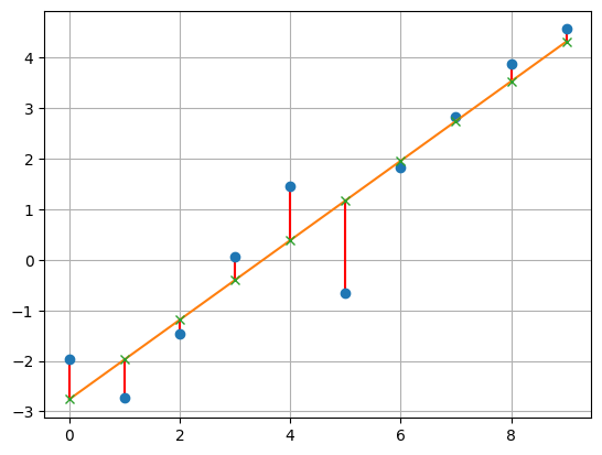
Here's a larger example. Suppose this is our set of points.
| $t$ | $b$ |
|---|---|
| 0 | -1.97470391 |
| 1 | -2.73770318 |
| 2 | -1.4711225 |
| 3 | 0.06603995 |
| 4 | 1.46591915 |
| 5 | -0.65201352 |
| 6 | 1.81753915 |
| 7 | 2.83185776 |
| 8 | 3.87709595 |
| 9 | 4.56430677 |
Because this is quite long, we'll proceed by computation only.
    >>> t = np.arange(10)
    >>> b = np.array([-1.97470391, -2.73770318, -1.4711225 ,  0.06603995,
    ...                1.46591915, -0.65201352,  1.81753915,  2.83185776,
    ...                3.87709595,  4.56430677])
    >>> A = np.ones((10, 2))
    >>> A[:,1] = t
    >>> A
    array([[1., 0.],
           [1., 1.],
           [1., 2.],
           [1., 3.],
           [1., 4.],
           [1., 5.],
           [1., 6.],
           [1., 7.],
           [1., 8.],
           [1., 9.]])
    >>> A.T @ A
    array([[ 10.,  45.],
           [ 45., 285.]])
    >>> A.T @ b
    array([ 7.78721562, 99.94554842])
    >>> x = np.linalg.solve(A.T @ A, A.T @ b)
    >>> x
    array([-2.76144634,  0.78670398])
    >>> A @ x
    array([-2.76144634, -1.97474236, -1.18803838, -0.4013344 ,  0.38536957,
            1.17207355,  1.95877753,  2.74548151,  3.53218548,  4.31888946])
    >>> b - A @ x
    array([ 0.78674243, -0.76296082, -0.28308412,  0.46737435,  1.08054958,
           -1.82408707, -0.14123838,  0.08637625,  0.34491047,  0.24541731])
We've illustrated this with lines of best fit, which are just 1-dimensional spaces. The natural question is whether we can generalize this to more dimensions. The answer is yes. For instance, suppose that our dataset has two features:
| $t_1$ | $t_2$ | $b$ |
|---|---|---|
| 0 | -2 | 9 |
| 1 | 3 | 23 |
| 2 | -24 | 1 |
| 3 | 13 | -5 |
| 4 | -3 | -12 |
Then the linear function we want to model would be something like $b = x_0 + x_1t_1 + x_2t_2$. But this linear function describes a plane, so what we'd be doing is trying to find is a plane of best fit. Then we end up with a matrix $A$ that has rows of the form $\begin{bmatrix} 1 & t_{1,i} & t_{2,i} \end{bmatrix}$ and $\mathbf{\hat x} = \begin{bmatrix} x_0 \\ x_1 \\ x_2 \end{bmatrix}$. So our above data table turns into \[A = \begin{bmatrix} 1 & 0 & 2 \\ 1 & 1 & 3 \\ 1 & 2 & -24 \\ 1 & 3 & 13 \\ 1 & 4 & -3 \end{bmatrix}, \mathbf b = \begin{bmatrix} 9 \\ 23 \\ 1 \\ -5 \\ -12 \end{bmatrix}.\] It's not hard to see how we can add on more features to our model and we end up describing higher-dimensional spaces to predict our variable of interest, $b$.
    >>> t1 = np.arange(5)
    >>> t2 = np.array([2, 3, -24, 13, -3])
    >>> y = np.array([9, 23, 1, -5, -12])
    >>> A = np.ones((5, 3))
    >>> A[:,1] = t1
    >>> A[:,2] = t2
    >>> A
    array([[  1.,   0.,   2.],
           [  1.,   1.,   3.],
           [  1.,   2., -24.],
           [  1.,   3.,  13.],
           [  1.,   4.,  -3.]])
    >>> A.T @ A
    array([[  5.,  10.,  -9.],
           [ 10.,  30., -18.],
           [ -9., -18., 767.]])
    >>> A.T @ y
    array([ 16., -38.,  34.])
    >>> x = np.linalg.solve(A.T @ A, A.T @ y)
    >>> x
    array([17.3505594 , -7.        ,  0.08364411])
Since this is in 3D, it is possible to plot, but it is admittedly beyond the limits of my current knowledge of matplotlib and skill at sketching. What we should see is a plane where $\mathbf b$ is associated with the "vertical" at each point $(t_1, t_2)$ and $\mathbf e$ is the distance from each point to its respective location on the plane.
In this setup, we notice that $x_1$ and $x_2$ plays the role of "weighting" the features $t_1$ and $t_2$ in the way that we talked about when we first introduced the dot product. And in fact, this is exactly what we are getting when we put everything together.
What's nice about this is how simply by assuming that there's a linear relationship in our data gives us enough bones to put together to get a model like this.