Now, how do we generalize this to a subspace of arbitrary dimension? Simple—just do the same thing but for each "dimension". Here, we see why we want a basis for our subspace—each basis vector represents a "direction" or dimension of the subspace. So if we want to project a vector onto the subspace, we simply metaphorically project the vector onto each line described each basis vector. Practically speaking, this means that our projection is going to be a linear combination of these basis vectors.
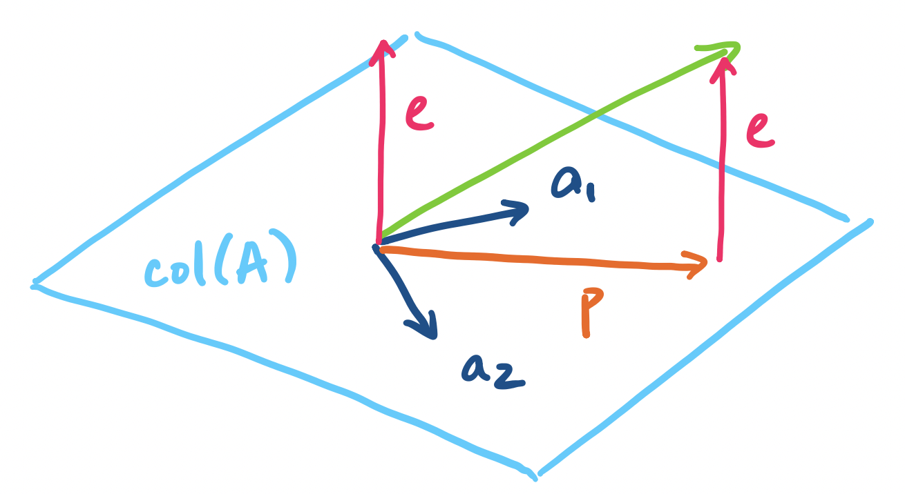
Let $\mathbf a_1, \dots, \mathbf a_n$ be vectors in $\mathbb R^m$ that span a subspace $S$. Then the projection of $\mathbf b$ onto $S$ is the vector $\mathbf p = \hat x_1 \mathbf a_1 + \cdots + \hat x_n \mathbf a_n$ in $S$ that is closest to $\mathbf b$. By closest, we mean that the length of the error vector $\mathbf e = \mathbf p - \mathbf b$ is minimized.
Why does this work? Recall that the vectors in the basis are all independent. We can think of each basis vector as being the description of a particular "direction" in the space and because they are independent, they describe the only way to head in that direction. So naturally, a linear combination of the basis vectors can be thought of as saying "proceed in the direction $\mathbf a_1$ by $x_1$ amount, then go in direction $\mathbf a_2$ by $x_2$ amount", and so on.
This means that we will be doing the same projection computation that we've been doing but on all the basis vectors. This seems like a pain to do, but as usual, our trick for working with multiple vectors at once is to throw all of them into a single matrix and express all the computations as a matrix product. Then it becomes clear that our $\hat x_i$'s are the components of a vector $\mathbf{\hat x}$ that describes the desired linear combination of the basis vectors.
We generalize our setting: instead of a single line defined by a vector $\mathbf a$, we project our vector onto a subspace with basis $\mathbf a_1, \dots, \mathbf a_n$. We take these basis vectors and put them together into a single matrix $A = \begin{bmatrix} \big\vert & & \big\vert \\ \mathbf a_1 & \cdots & \mathbf a_n \\ \big\vert & & \big\vert \end{bmatrix}$. This means our projection will be given by $\mathbf p = A \mathbf{\hat x}$, where $\mathbf{\hat x}$ is a vector $\begin{bmatrix} \hat x_1 \\ \hat x_2 \\ \vdots \\ \hat x_n \end{bmatrix}$, not just a scalar (which explains why $\mathbf{\hat x}$ is written the way it is).
First, we make an observation about the error vector again.
Let $\mathbf p$ be the projection of $\mathbf b$ onto a subspace with basis vectors $\mathbf a_1, \dots, \mathbf a_n$. Then the error vector $\mathbf e = \mathbf b - \mathbf p$ is perpendicular to all of the basis vectors.
Why is the error perpendicular to the subspace? Intuitively, the error vector forms a line straight "down" to the subspace—the shortest and fastest way to get from the vector $\mathbf b$ to the subspace. In other words, this minimizes $\|\mathbf e\|$ where $\mathbf e = \mathbf b - \mathbf p_i$ for each projection vector $\mathbf p_i$.
This means that for each basis vector $\mathbf a_i$ for our subspace, we must have $\mathbf a_i^T (\mathbf b - \mathbf a_i \hat x_i) = 0$. Then we can apply the same reasoning as with projection to a line above, giving us \[\mathbf p_i = \mathbf a_i \hat x_i = \mathbf a_i \frac{\mathbf a_i^T \mathbf b}{\mathbf a_i^T \mathbf a_i}.\]
Now, recall that all of these basis vectors are columns of the matrix $A$. This means that:
So we take all of these vector products and instead think of them as matrix products instead: \[\begin{bmatrix} \rule[.5ex]{1.5em}{0.5pt} & \mathbf a_1^T & \rule[.5ex]{1.5em}{.5pt} \\ & \vdots & \\ \rule[.5ex]{1.5em}{0.5pt} & \mathbf a_n^T & \rule[.5ex]{1.5em}{.5pt} \end{bmatrix} \left( \begin{bmatrix} b_1 \\ \vdots \\ b_n \end{bmatrix} - \begin{bmatrix} \big\vert & & \big\vert \\ \mathbf a_1 & \cdots & \mathbf a_n \\ \big\vert & & \big\vert \end{bmatrix} \begin{bmatrix} \hat x_1 \\ \vdots \\ \hat x_n \end{bmatrix} \right) = \begin{bmatrix} 0 \\ \vdots \\ 0 \end{bmatrix}\] Or more succinctly, \[A^T(\mathbf b - A\mathbf{\hat x}) = \mathbf 0.\]
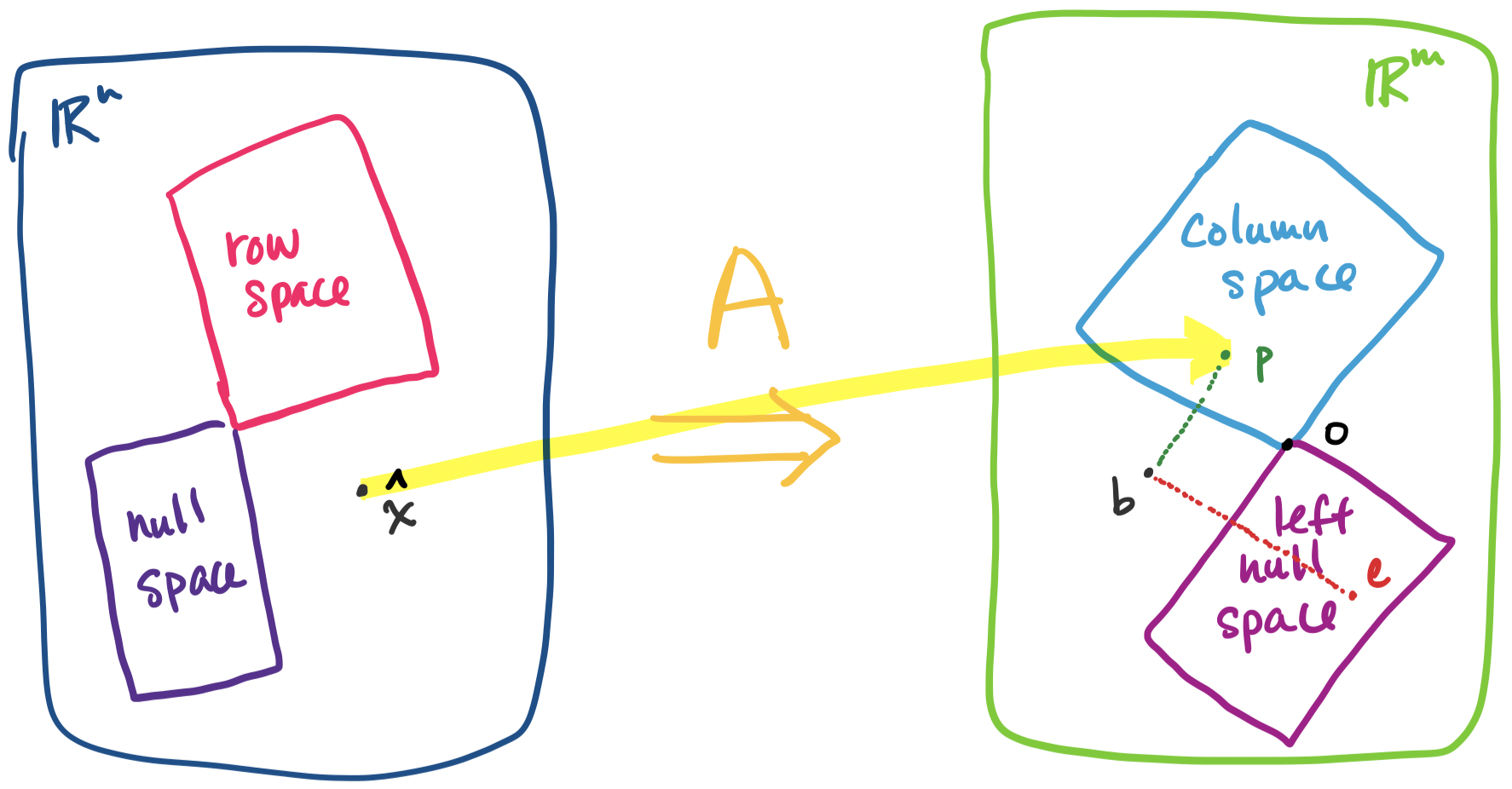
Now it becomes clear why we wrote $\mathbf a^T$ and $\mathbf{\hat x}$. We arrived at all of this geometrically, but we should take a step back and examine this closely. Recall that $\mathbf b - A \mathbf{\hat x} = \mathbf e$ by definition. So our equation above tells us \[A^T \mathbf e = \mathbf 0.\] In other words, $\mathbf e$ is in the left nullspace of $A$! This makes sense because $\mathbf e$ is orthogonal to the column space of $A$, so by orthogonal complements, this can be the only outcome.
But recall our discussion of the decomposition of $\mathbf x = \mathbf x_r + \mathbf x_n$ where $\mathbf x$ is any vector in $\mathbb R^n$, $\mathbf x_r$ is a row space vector, and $\mathbf x_n$ is a null space vector. We have a similar outcome here: $\mathbf b = \mathbf p + \mathbf e$, where $\mathbf b$ is any vector in $\mathbb R^m$, $\mathbf p$ is a vector in the column space, and $\mathbf e$ is a vector in the left null space. Everything fits together.
If we recall the one-dimensional case, we had the equation \[\mathbf a^T (\mathbf b - \mathbf a \mathbf{\hat x}) = \mathbf 0 \] Notice that when we return to the multi-dimensional case, we swap out the single basis vector $\mathbf a$ for a matrix $A$ with columns $\mathbf a_1, \dots, \mathbf a_n$ which are the basis vectors for $S$ and $\mathbf{\hat x}$ is now a vector. We get that \[A^T (\mathbf b - A \mathbf{\hat x}) = \mathbf 0 \]
From here, we need to find $\mathbf{\hat x}$ to find the projection $\mathbf p = A\mathbf{\hat x}$. First, we rearrange the equation to give us \[A^TA\mathbf{\hat x} = A^T \mathbf b.\] The above equation suggests that if we could get rid of $A^T$ on both sides, we'd be good. We observe that \[\mathbf{\hat x} = (A^T A)^{-1} A^T \mathbf b.\] This is just the matrix version of $\mathbf{\hat x} = \frac{\mathbf a^T \mathbf b}{\mathbf a^T \mathbf a} = (\mathbf a^T \mathbf a)^{-1} \mathbf a^T \mathbf b$.
This seems fine, but there should be a red flag going off in your head: why are we allowed to do this? Let's go through the possible pitfalls:
We need to find $\mathbf{\hat x}$ in order to find the projection $\mathbf p = A \mathbf{\hat x}$. We have \[\mathbf{\hat x} = (A^T A)^{-1} A^T \mathbf b.\]
Now, this suggests that we are going to have to compute the inverse. But we didn't need to do this before to solve a system of linear equations and we are not going to start now. If all we want is the vector $\mathbf{\hat x}$, then we just need to solve the system $A^TA \mathbf{\hat x} = A^T \mathbf b$. However, this identity will be useful to play around with, so we will continue to refer to it for now.
Once we have found $\mathbf{\hat x}$, it is not hard to find the projection vector $\mathbf p$: \[\mathbf p = A \mathbf{\hat x} = A(A^T A)^{-1} A^T \mathbf b.\] Of course, this is just what we get via straightforward substitution from our previous result. We make one more observation to get the projection matrix: \[P = A(A^T A)^{-1} A^T.\] Again, this is just the matrix that we multiply by $\mathbf b$ from the previous equation.
If we take a closer look at what we've done, we see that it is essentially the same as what we did for projection on a line: \[\mathbf p = \mathbf a \mathbf{\hat x} = \mathbf a \frac{\mathbf a^T \mathbf b}{\mathbf a^T \mathbf a} = \mathbf a (\mathbf a ^T \mathbf a )^{-1} \mathbf a ^T \mathbf b.\]
Suppose we want to project $\mathbf b = \begin{bmatrix} 3 \\ 1 \\ 5 \end{bmatrix}$ onto the subspace spanned by the vectors $\begin{bmatrix} 0 \\ 1 \\ 2 \end{bmatrix}$ and $\begin{bmatrix} 1 \\ 1 \\ 1 \end{bmatrix}$. First, we put our vectors into a matrix $A = \begin{bmatrix} 1 & 0 \\ 1 & 1 \\ 1 & 2 \end{bmatrix}$. Now, the problem becomes projecting $\mathbf b$ onto the column space of $A$. With $A$, we compute $A^TA$, \[\begin{bmatrix} 1 & 1 & 1 \\ 0 & 1 & 2 \end{bmatrix} \begin{bmatrix} 1 & 0 \\ 1 & 1 \\ 1 & 2 \end{bmatrix} = \begin{bmatrix} 3 & 3 \\ 3 & 5 \end{bmatrix}.\] Then we compute $A^T \mathbf b$, \[\begin{bmatrix} 1 & 1 & 1 \\ 0 & 1 & 2 \end{bmatrix} \begin{bmatrix} 3 \\ 1 \\ 5 \end{bmatrix} = \begin{bmatrix} 9 \\ 11 \end{bmatrix}.\]
This gives us: \[\begin{bmatrix} 3 & 3 \\ 3 & 5 \end{bmatrix} \begin{bmatrix} \hat x_1 \\ \hat x_2 \end{bmatrix} = \begin{bmatrix} 9 \\ 11 \end{bmatrix},\] This is just the system of linear equations \begin{align*} 3\hat x_1 + 3 \hat x_2 &= 9 \\ 3\hat x_1 + 5 \hat x_2 &= 11 \end{align*} You can solve this system however you like. From this, it's not too hard to see that $\mathbf{\hat x} = \begin{bmatrix} 2 \\ 1 \end{bmatrix}$.
    >>> b = np.array([3, 1, 5])
    >>> A = np.array([[1, 0], [1, 1], [1, 2]])
    >>> A.T @ A
    array([[3, 3],
           [3, 5]])
    >>> A.T @ b
    array([ 9, 11])
    >>> np.linalg.solve(A.T @ A, A.T @ b)
    array([2., 1.])
This then gives us the projection $\mathbf p = A \mathbf{\hat x}$, which is \[\begin{bmatrix} 1 & 0 \\ 1 & 1 \\ 1 & 2 \end{bmatrix} \begin{bmatrix} 2 \\ 1 \end{bmatrix} = 2 \begin{bmatrix} 1 \\ 1 \\ 1 \end{bmatrix} + \begin{bmatrix} 0 \\ 1 \\ 2 \end{bmatrix} = \begin{bmatrix} 2 \\ 3 \\ 4 \end{bmatrix}.\]
    >>> x = np.linalg.solve(A.T @ A, A.T @ b)
    >>> A @ x
    array([2., 3., 4.])
Finally, the projection matrix is $P = A(A^TA)^{-1} A^T$, which is $\frac 1 6 \begin{bmatrix} 5 &2 &-1 \\ 2 & 2 & 2 \\ -1 & 2 & 5 \end{bmatrix}$:
    >>> P = A @ np.linalg.inv(A.T @ A) @ A.T
    >>> P
    array([[ 0.83333333,  0.33333333, -0.16666667],
           [ 0.33333333,  0.33333333,  0.33333333],
           [-0.16666667,  0.33333333,  0.83333333]])
    >>> P @ b
    array([2., 3., 4.])
Let's return to our original problem: we want to solve $A \mathbf x = \mathbf b$ but $\mathbf b$ is not in the column space of $A$. This means we want to find $\mathbf x$ that gives us the vector in the column space of $A$ that is closest to $\mathbf b$. This vector is $\mathbf p = A \mathbf{\hat x}$, the projection of $\mathbf b$ onto the column space of $A$.
How do we find $\mathbf{\hat x}$? This depends on the error vector $\mathbf e = \mathbf b - A \mathbf{\hat x}$. Since we want $\mathbf b$ and $\mathbf p$ to be as close as possible, we must have that $\mathbf e$ that minimizes $\|\mathbf e\|$, which means it is perpendicular to the column space. But this means $\mathbf e$ is in the left null space of $A$! This gives us \[A^T\mathbf e = A^T (\mathbf b - A \mathbf{\hat x}) = \mathbf 0,\] so $A^T A \mathbf{\hat x} = A^T \mathbf b$.
In summary, suppose we want to compute the projection of a vector onto a subspace.