Suppose we have a vector and we know that some part of it belongs to a subspace. How can we figure out what that piece is? This brings us to the idea of projection.
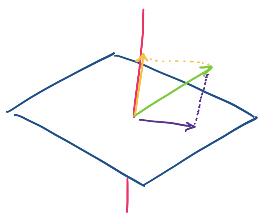
The usual analogy for projection is of a light pointed at some object, which casts a shadow on a surface. For example, a shadow on a wall, or your shadow created by a light pointing at you from above. The shadow is the projection of the object onto the surface, a plane, which we can think of as our subspace. We get a nice visual when we imagine this in $\mathbb R^3$.
Consider a vector $\mathbf v$ in $\mathbb R^3$. We want to consider projections on the $x,y$-plane and the $z$ axis. It's clear that if $\mathbf v = \begin{bmatrix} x \\ y \\ z \end{bmatrix}$, then our two projections are $\begin{bmatrix} x \\ y \\ 0 \end{bmatrix}$ and $\begin{bmatrix} 0 \\ 0 \\ z \end{bmatrix}$.
As usual, we can encode projections as matrices. For projection onto the $x,y$-plane, we have $\begin{bmatrix} 1 & 0 & 0 \\ 0 & 1 & 0 \\ 0 & 0 & 0 \end{bmatrix}$ and $\begin{bmatrix} 0 & 0 & 0 \\ 0 & 0 & 0 \\ 0 & 0 & 1 \end{bmatrix}$ for projection onto the $z$-axis.
We notice that this works out quite nicely because our two chosen subspaces happen to be orthogonal complements.
This is the easy case. But what if our subspaces are not perfectly aligned with the standard axes? What we want is to generalize this for higher dimensional spaces and for subspaces that are not perfectly aligned to our standard axes.
This seems like a geometric exercise, but, projections are neither just an idea that works only in geometry nor is it just an abstract concept when we move to higher-dimensional spaces. Among a whole host of applications, one that we can imemediately discuss is how we implicitly apply the idea of projections every time we take some high-dimensional data and attempt to visualize it.
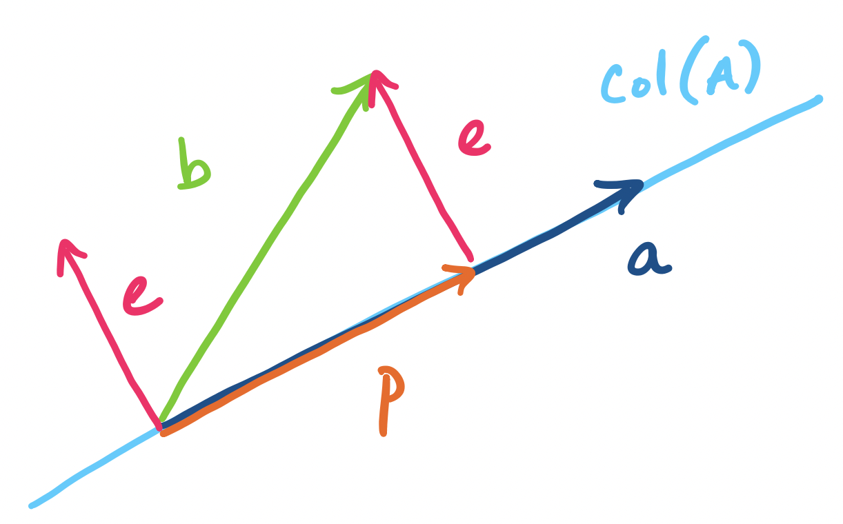
We begin with the simplest subspace to project onto: a line. Lines are defined by a single vector, which we denote by $\mathbf a$. We will project a vector $\mathbf b$ onto the line going through $\mathbf a$. The projection is called $\mathbf p$.
There are a few things to note here.
So how do we find $\mathbf{\hat x}$? Ideally, we would like to find the vector on the line that is closest to $\mathbf b$. In order to this, we need to talk about the distance between $\mathbf b$ and the possible projection $\mathbf p$. Recall that the distance between $\mathbf b$ and $\mathbf p$ is the quantity $\|\mathbf b - \mathbf p\|$. This vector that we've defined is $\mathbf e = \mathbf b - \mathbf p$ is called the error, since it quantifies how "far" $\mathbf b$ is outside of the subspace spanned by $\mathbf a$.
Our goal is to find $\mathbf p$ so that $\|\mathbf e\| = \|\mathbf b - \mathbf p\|$ is minimized. In other words, what is the shortest distance between $\mathbf b$ and $\mathbf p$? Visually, we can try to slide along the line defined by $\mathbf a$. What we'll find is that $\|\mathbf e\|$ is shortest when it is orthogonal to $\mathbf a$.
Based on this observation, we can find $\mathbf{\hat x}$.
The projection $\mathbf p$ of $\mathbf b$ onto $\mathbf a$ is \[\mathbf p = \mathbf a \mathbf{\hat x} = \mathbf a \frac{\mathbf a^T \mathbf b}{\mathbf a^T \mathbf a}.\]
By definition, we know that $\mathbf p = \mathbf a \mathbf{\hat x}$ for some scalar $\mathbf{\hat x}$. We observe that $\mathbf e = \mathbf b - \mathbf a \mathbf{\hat x}$ is perpendicular to $\mathbf a$ when $\|\mathbf e\|$ is minimized. So we have \begin{align*} \mathbf a \cdot \mathbf e &= 0 \\ \mathbf a \cdot (\mathbf b - \mathbf a \mathbf{\hat x}) &= 0 \\ \mathbf a \cdot \mathbf b - (\mathbf a \cdot \mathbf a)\mathbf{\hat x} &= 0 \\ \mathbf{\hat x} &= \frac{\mathbf a \cdot \mathbf b}{\mathbf a \cdot \mathbf a} \end{align*}
In other words, $\mathbf{\hat x} = \frac{\mathbf a^T \mathbf b}{\mathbf a^T \mathbf a}$.
Let's start with a relatively simple example. Let $\mathbf a = \begin{bmatrix} 2 \\ 1 \end{bmatrix}$. We want to project $\mathbf b = \begin{bmatrix} 1 \\ 2 \end{bmatrix}$ onto $\mathbf a$.
To compute $\mathbf p = \mathbf a \mathbf{\hat x}$, we need to compute $\mathbf{\hat x}$. We have
\[ \mathbf a^T \mathbf a = 2^2 + 1^2 = 5\]
\[ \mathbf a^T \mathbf b = 2 \cdot 1 + 1 \cdot 2 = 4\]
So $\mathbf{\hat x} = \frac 4 5$ and $\mathbf p =\frac 4 5 \mathbf a$.
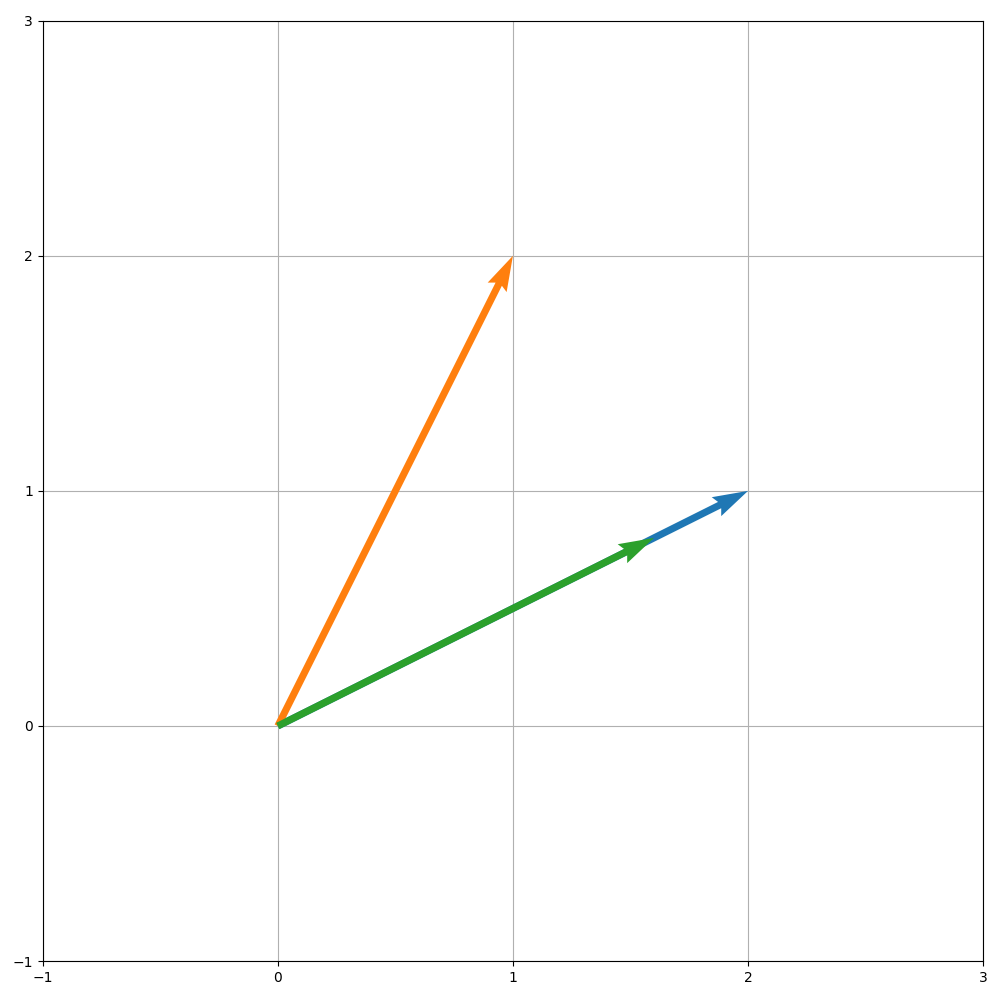
Now, we can continue and compute $\mathbf e = \mathbf b - \mathbf p$. This is
\[ \mathbf e = \mathbf b - \mathbf p = \begin{bmatrix} 1 \\ 2 \end{bmatrix} - \begin{bmatrix} \frac 8 5 \\ \frac 4 5 \end{bmatrix} = \begin{bmatrix} -\frac 3 5 \\ \frac 6 5 \end{bmatrix}.\]
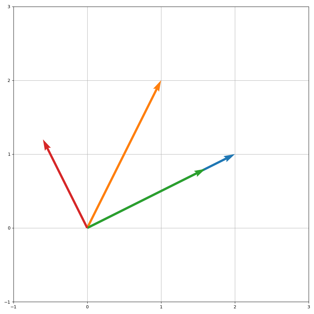
Visually, we can see that it is indeed the case that $\mathbf e$ is orthogonal to $\mathbf p$ and all the other vectors along the line described by $\mathbf a$. We can also verify this numerically: \[\mathbf a \cdot \mathbf e = 2 \cdot -\frac 3 5 + 1 \cdot \frac 6 5 = 0.\] Then we have \[\|\mathbf e \| = \sqrt{\left(-\frac 3 5\right)^2 + \left(\frac 6 5 \right)^2} = \sqrt{\frac{45}{25}} = \frac{3\sqrt5}{5}.\]
Here's an example in $\mathbb R^3$. Let $\mathbf b = \begin{bmatrix} 1 \\ -2 \\ 1 \end{bmatrix}$. We will project $\mathbf b$ onto $\mathbf a = \begin{bmatrix} 3 \\ 1 \\ 2 \end{bmatrix}$. We need to compute $\mathbf{\hat x}$ to get $\mathbf p$. We have \[\mathbf a^T \mathbf a = 3^2 + 1^2 + 2^2 = 14\] \[\mathbf a^T \mathbf b = 3 \cdot 1 + 1 \cdot -2 + 2 \cdot 1 = 3\] This gives $\mathbf{\hat x} = \frac{3}{14}$. So $\mathbf p = \begin{bmatrix} \frac{9}{14} \\ \frac{3}{14} \\ \frac{6}{14} \end{bmatrix}$.
    >>> b = np.array([1, -2, 1]).reshape(3,1)
    >>> a = np.array([3, 1, 2]).reshape(3,1)
    >>> a.T @ a
    array([[14]])
    >>> a.T @ b
    array([[3]])
    >>> x = (a.T @ b)/(a.T @ a)
    array([[0.21428571]])
    >>> x * a
    array([[0.64285714],
           [0.21428571],
           [0.42857143]])
We can verify this by considering the other definition for $\mathbf p$, that $\mathbf e = \mathbf b - \mathbf p$. We first compute \[\mathbf e = \begin{bmatrix} 1 \\ -2 \\ 1 \end{bmatrix} - \begin{bmatrix} \frac{9}{14} \\ \frac{3}{14} \\ \frac{6}{14} \end{bmatrix} = \begin{bmatrix} \frac{5}{14} \\ -\frac{31}{14} \\ \frac{8}{14} \end{bmatrix}.\] Then \[\mathbf e \cdot \mathbf a = 3 \cdot \frac{5}{14} - \frac{31}{14} + 2 \cdot \frac{8}{14} = 0,\] as desired.
    >>> p = x * a
    >>> e = b - p
    >>> e
    array([[ 0.35714286],
           [-2.21428571],
           [ 0.57142857]])
    >>> e.T @ a
    array([[0.]])
Recall that we can view projection as a transformation, so we can define a matrix that will project a vector onto a particular subspace. To do this for a line, we use what we just did and work backwards, noting that we should have $\mathbf p = P \mathbf b$.
Let $\mathbf p$ be the projection of $\mathbf b$ on $\mathbf a$. Then $\mathbf p = P \mathbf b$, where $P = \frac{\mathbf a \mathbf a^T}{\mathbf a^T \mathbf a}$.
To get our projection matrix $P$, we simply take $\mathbf p = \mathbf a \mathbf{\hat x}$ and rearrange it. We have \begin{align*} \mathbf p &= \mathbf a \mathbf{\hat x} \\ &= \mathbf a \frac{\mathbf a^T \mathbf b}{\mathbf a^T \mathbf a} \\ &= \frac{\mathbf a \mathbf a^T}{\mathbf a^T \mathbf a} \mathbf b \\ &= \frac{1}{\mathbf a^T \mathbf a}(\mathbf a \mathbf a^T) \mathbf b \\ \end{align*}
This tells us that our projection matrix $P$ is a rank 1 matrix $\mathbf a \mathbf a^T$, that is scaled by $\mathbf a \cdot \mathbf a$.
From our earlier example, we had $\frac{1}{\mathbf a^T \mathbf a} = \frac{1}{14}$. Then we compute the rank 1 matrix \[\mathbf a \mathbf a^T = \begin{bmatrix} 9 & 3 & 6 \\ 3 & 1 & 2 \\ 6 & 2 & 4 \end{bmatrix}.\] Together, this gives us \[P = \frac{\mathbf a \mathbf a^T}{\mathbf a^T \mathbf a} = \frac{1}{14} \begin{bmatrix} 9 & 3 & 6 \\ 3 & 1 & 2 \\ 6 & 2 & 4 \end{bmatrix} = \begin{bmatrix} \frac{9}{14} & \frac{3}{14} & \frac{6}{14} \\ \frac{3}{14} & \frac{1}{14} & \frac{2}{14} \\ \frac{6}{14} & \frac{2}{14} & \frac{4}{14} \end{bmatrix}.\]
    >>> a @ a.T
    array([[9, 3, 6],
           [3, 1, 2],
           [6, 2, 4]])
    >>> P = 1/(a.T @ a) * a @ a.T
    >>> P
    array([[0.64285714, 0.21428571, 0.42857143],
           [0.21428571, 0.07142857, 0.14285714],
           [0.42857143, 0.14285714, 0.28571429]])
    >>> P @ b
    array([[0.64285714],
           [0.21428571],
           [0.42857143]])
Notice that the projection matrix $P$ doesn't depend on $\mathbf b$ at all. The projection matrix is for projecting onto the line, which means that $P \mathbf d$ will give us the projection of some other vector $\mathbf d$ onto the line going through $\mathbf a$.