The Fundamental Theorem of Linear algebra tells us that for a matrix $A$, its row space and null space are orthogonal complements and its column space and left null space are orthogonal complements.
There is an important consequence that we get from this:
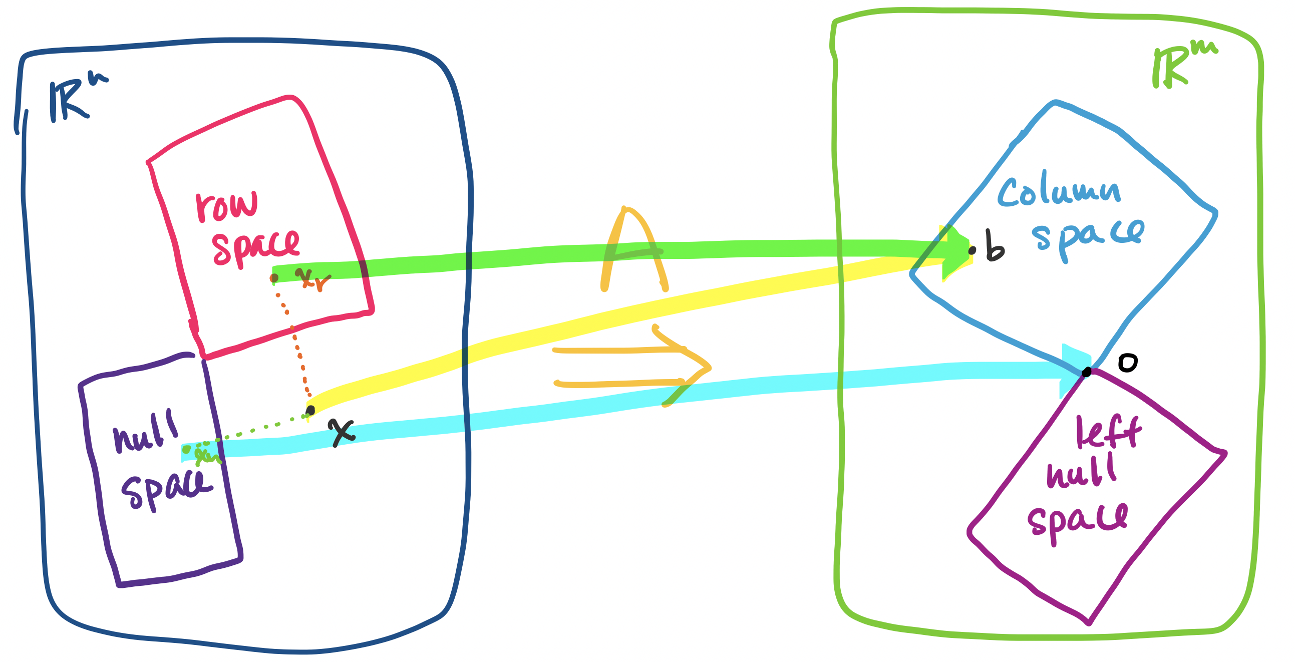
Let $A$ be an $m \times n$ matrix. For the linear equation $A \mathbf x = \mathbf b$, every solution $\mathbf x$ can be described as a vector $\mathbf x = \mathbf x_r + \mathbf x_n$, where $\mathbf x_r$ is in the row space of $A$ and is unique for $\mathbf b$ and $\mathbf x_n$ is a vector from the null space of $A$.
How does this help us? Consider the example of $A$ as an operation that transform a vector $\mathbf x$ in $\mathbb R^n$ into a vector $\mathbf b$ in $\mathbb R^m$. When this occurs, some part of the information in this vector gets "lost" or "flattened"—this is the part of the vector in the null space. However, up until now, we haven't had a way to talk about how to 'get' this part of the vector.
It is orthogonality, which describes how the null space of a matrix is oriented with respect to its row space, that will give us the tools to do so.
Let $A$ be an $m \times n$ matrix and let $\mathbf x$ be a vector in $\mathbb R^n$. Then it can be written as the sum of two vectors $\mathbf x_r + \mathbf x_n$, where $\mathbf x_r$ is in the row space of $A$ and $\mathbf x_n$ is in the null space of $A$.
Consider a basis $\mathbf u_1, \dots, \mathbf u_r$ for the row space of $A$ and a basis $\mathbf v_1, \dots, \mathbf v_{n-r}$ for the null space of $A$. A basis for the row space has $r$ vectors, where $r$ is the rank of $A$, and a basis for the null space of $A$ has $n-r$ vectors. Therefore, we have $n$ vectors in total.
Since each set of vectors is a basis, each set is linearly independent. Since the two subspaces are orthogonal to each other, all of the vectors are linearly independent. Since our set of $n$ vectors is linearly independent, they must span $\mathbb R^n$. Therefore, they form a basis for $\mathbb R^n$.
Since the bases for the row and null spaces forms a basis for $\mathbb R^n$, every vector $\mathbf x$ can be written as a linear combination of these basis vectors, \[\mathbf x = a_1 \mathbf u_1 + \cdots a_r \mathbf u_r + b_1 \mathbf v_1 + \cdots + b_{n-r} \mathbf v_{n-r}.\] Then by grouping the terms, we can write $\mathbf x$ as \begin{align*} \mathbf x &= \overbrace{a_1 \mathbf u_1 + \cdots a_r \mathbf u_r}^{\text{row space vector}} + \overbrace{b_1 \mathbf v_1 + \cdots + b_{n-r} \mathbf v_{n-r}}^{\text{null space vector}} \\ &= \mathbf x_r + \mathbf x_n \end{align*}
If you look at the above proof carefully, you'll notice that we never actually use the fact that we have the row space and the null space of a matrix. The only way we use this information is to conclude that they are orthogonal complements—that they have the right dimensions and orientation with respect to each other. So in fact, we could replace "row space" and "null space" with any two subspaces which are orthogonal complements and use the same proof. This means that we can actually say something stronger.
Let $U$ and $V$ be subspaces of $\mathbb R^n$ that are orthogonal complements and let $\mathbf x$ be a vector in $\mathbb R^n$. Then $\mathbf x$ can be written as the sum of two vectors $\mathbf u + \mathbf v$, where $\mathbf u$ is a vector in $U$ and $\mathbf v$ is a vector in $V$.
If we proved this first, we could get that every vector in $\mathbb R^n$ can be written as a vector from the row space and a vector from the null space. Then it's not hard to see that we also have that every vector in $\mathbb R^m$ can be written as a vector from the column space and a vector from the left null space.
This then allows us to prove that if $A \mathbf x = \mathbf b$ has a solution, then there is exactly one solution $\mathbf x$ that belongs to the row space.
Suppose that there were another vector $\mathbf y$ from the row space such that $A \mathbf y = \mathbf b$. Then we have $A \mathbf x - A \mathbf y = A (\mathbf x - \mathbf y) = \mathbf 0$.
Since we said that both $\mathbf x$ and $\mathbf y$ are in the row space of $A$ and the row space is a subspace, this means that $\mathbf x - \mathbf y$ is also a vector in the row space. But since $A(\mathbf x - \mathbf y) = \mathbf 0$, $\mathbf x - \mathbf y$ is a vector in the null space. But the only vector in both the row space and the null space can only be $\mathbf 0$. So this tells us $\mathbf x = \mathbf y$.
As a reminder, recall that this is not the particular solution. The particular solution is actually already some combination of a row space vector and null space vector. One can test this: try to see if you can describe a particular solution using rows of the row-reduced echelon form. Alternatively, see if it is orthogonal to a vector from the null space.
One other consequence of this is that it tells us that every vector in the column space can be paired off with a vector from the row space. This allows us to conclude that the two spaces are exactly the same size. Even though this seems feasible, as the two spaces have the same dimension, $r$, the rank of the matrix, it's not totally obvious that the two have to contain since the exact same number of vectors. After all, there are infinitely many vectors in both. But this correspondence tells us exactly this: there is exactly one vector in the row space for each vector in the column space and vice-versa.
As an aside, it's this technique, pairing off elements, that allows mathematicians to show things like the fact that there are exactly as many integers as there are pairs of integers but that there are strictly more real numbers than there are integers.
Now, consider the following example.
Let $A = \begin{bmatrix} 3 & 1 \\ 9 & 3 \end{bmatrix}$ and consider the vector $\begin{bmatrix} 7 \\ 9 \end{bmatrix}$. The rref of $A$ is $\begin{bmatrix} 1 & \frac 1 3 \\ 0 & 0 \end{bmatrix}$, which gives a null space spanned by $\begin{bmatrix} -\frac 1 3 \\ 1 \end{bmatrix}$. Then we can write $\begin{bmatrix} 7 \\ 9 \end{bmatrix} = \begin{bmatrix} 9 \\ 3 \end{bmatrix} + \begin{bmatrix} -2 \\ 6 \end{bmatrix}$: the vector $\begin{bmatrix} 9 \\ 3\end{bmatrix}$ is from the row space (in fact, it's the second row) and $\begin{bmatrix} -2 \\ 6 \end{bmatrix}$ is from the null space (it is $6 \begin{bmatrix} -\frac 1 3 \\ 1 \end{bmatrix}$).
A problem with this very useful property at this point is it doesn't tell us how to split up our vector into these parts, only that we can. The example above was simple enough that we could just try some values and luck out. However, this is not a strategy that will work for anything non-trivial.
This becomes important when we consider the other side of the picture we've drawn. Though we've been occupied with $\mathbb R^n$ and the row space and null space of $A$, it's actually $\mathbb R^m$ and the column space and left null space that will occupy our attention at this point.
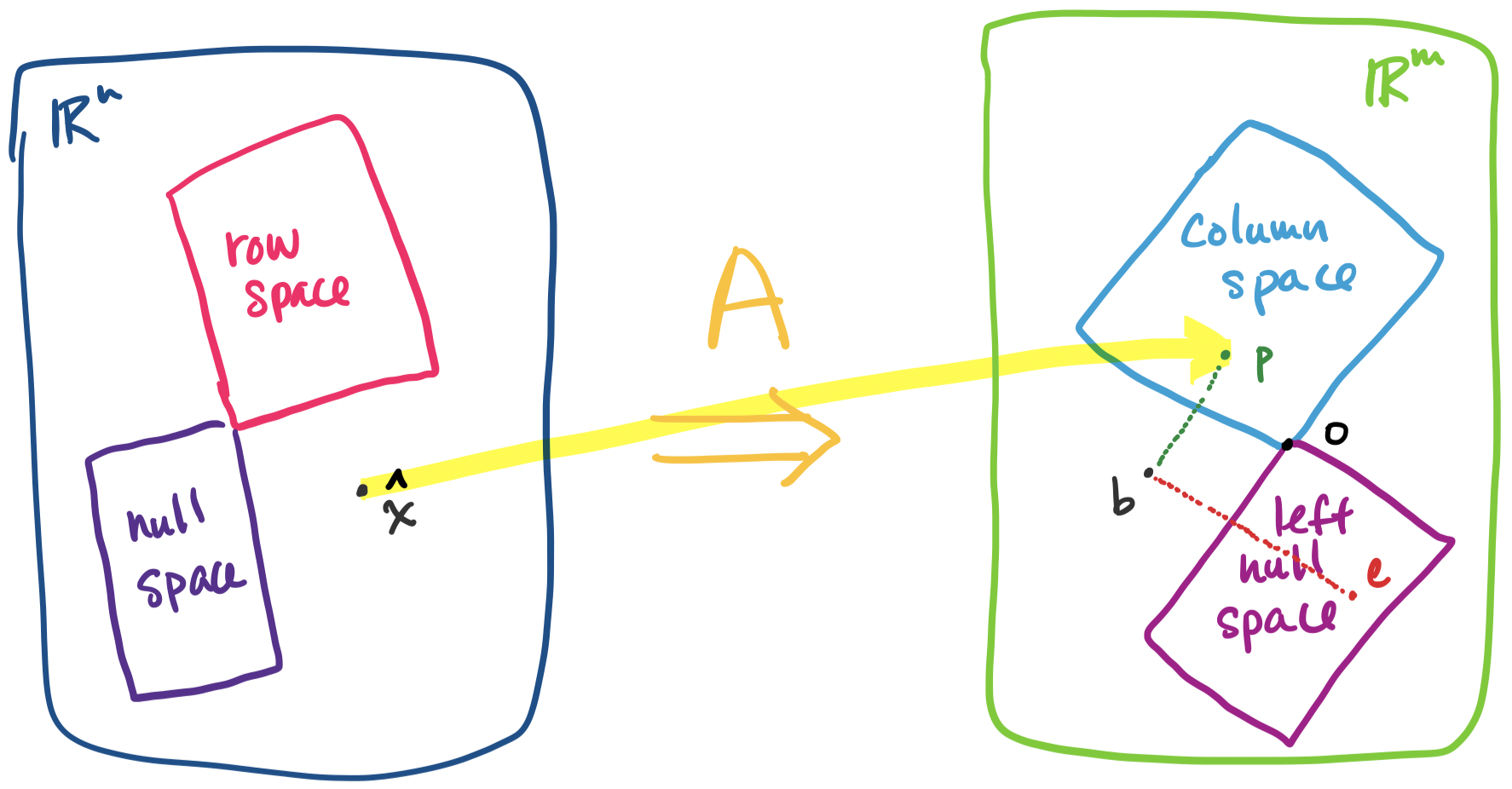
So far, when considering solutions to $A \mathbf x = \mathbf b$, we have dealt with the one solution case ($A$ has independent columns) and the infinite solution case ($A \mathbf x$ contains free variables). The remaining case is that $A \mathbf x = \mathbf b$ has no solutions. We've seen that the rref of $A$ in this case contains zero rows, but in the language of subspaces, this is the case when $\mathbf b$ is outside of the column space of $A$.
This scenario comes up often in real applications: we have a new object that we would like to interpret with respect to our existing dataset but it is different enough that it lies outside of the spaces we've defined. Another scenario involves trying to describe a space that is simpler than the actual dataset—this will necessarily put some points in the set outside of the simpler space.
It is here that the subspaces in $\mathbb R^m$ come into play. We've just seen that every vector in $\mathbb R^m$ can be described as a combination of two vectors: one from the column space and one from the left null space.
A promising idea is to try to figure out the relationship between each vector and its column space vector. This leads us to the search for an idea that will allow us to systematically find the components of vectors that lie in subspaces of interest.