We have seen the column space, the row space, and the null space of a matrix. However, there is an asymmetry: the row space and null space are in the same vector space, but the column space is on its own. Furthermore, the dimensions of the row space and null space are complementary, while the column space is on its own.
But if the row space of $A$ is just the column space of $A^T$, what if we did the same trick and took the null space of $A^T$. This is called the left null space of $A$.
The left nullspace of an $m \times n$ matrix $A$ is the set of vectors that satisfy $A^T \mathbf y = \mathbf 0$. It is a subspace of $\mathbb R^m$.
Why is this called the left nullspace of $A$? First, let's introduce a notational trick. We are used to viewing vectors as vertical columns. But what if we treat a vector in $\mathbb R^n$ as an $n \times 1$ matrix? We get the following.
Let $\mathbf u$ and $\mathbf v$ be vectors in $\mathbb R^n$. Then $\mathbf u^T \mathbf v = \mathbf u \cdot \mathbf v$.
This actually isn't that strange—it's exactly what we do when we compute matrix products for each entry: every entry of $AB$ is the dot product of a row of $A$ with a column of $B$. We'll see it's this exact operation that makes it a nice way to generalize ideas from vectors to matrices.
However, beware that this doesn't translate completely cleanly to NumPy arrays. In particular, you can't transpose a 1D array.
    >>> u = np.array([7, 6, 5])
    >>> u.T
    array([7, 6, 5])
So in NumPy, the exact form of the vectors you're considering will make a difference. If you have two 1D arrays, you should write u @ v. But if you're dealing with a row vector and a column vector as 2D arrays, you will find the u.T @ v notation helpful. That said, what you get is not a scalar, but a 2D array containing a single entry.
    >>> u = np.array([[7], [6], [5]])
    >>> v = np.array([[9], [6], [1]])
    >>> u @ v
    ValueError: matmul: Input operand 1 has a mismatch in its core
    dimension 0, with gufunc signature (n?,k),(k,m?)->(n?,m?) (size 3
    is different from 1)
    >>> u.T
    array([[7, 6, 5]])
    >>> u.T @ v
    array([[104]])
Using this, we can rewrite the equation $A^T \mathbf y = \mathbf 0$ in terms of $A$ as $\mathbf y^T A = \mathbf 0$ since $(AB)^T = B^T A^T$. Since $A^T$ is a matrix, it's clear that it has a nullspace, so we can carry out the same proof to find that the left nullspace is a subspace. We will soon see why this subspace is important. But for now, this is our missing piece.
The left null space of $R$ has dimension $m-r$.
Let's use the example $R$ that we've been working with. Since we're dealing $R$, a matrix in rref, solving for its left nullspace is actually quite simple. We first see that we have \[R^T = \begin{bmatrix} 1 & 0 & 0 \\ 3 & 0 & 0 \\ 1 & 0 & 0 \\ 0 & 1 & 0 \\ 9 & 3 & 0 \end{bmatrix}.\]
    >>> R = np.array([[1, 3, 1, 0, 9], [0, 0, 0, 1, 3], [0, 0, 0, 0, 0]])
    >>> R.T
    array([[1, 0, 0],
           [3, 0, 0],
           [1, 0, 0],
           [0, 1, 0],
           [9, 3, 0]])
It's important to note that in order to find the basis for the left null space of $A$ that we must take the transpose, $A^T$ and obtain the row-reduced form of $A^T$, not obtain the row-reduced form $R$ of $A$ and take its transpose $R^T$. One clue that this makes a difference is our discussion from last time that the column space of $A$ is not preserved by elimination.
To see this, consider the matrix $A = \begin{bmatrix} 1 & 3 & 1 & 0 & 9 \\ 0 & 0 & 0 & 1 & 3 \\ 1 & 3 & 1 & 1 & 12 \end{bmatrix}$. The row-reduced form of this matrix is $R$, from above. However, $A^T = \begin{bmatrix} 1 & 0 & 1 \\ 3 & 0 & 3 \\ 1 & 0 & 1 \\ 0 & 1 & 1 \\ 9 & 3 & 12 \end{bmatrix}$. The row-reduced form of $A^T$ is $\begin{bmatrix} 1 & 0 & 1 \\ 0 & 1 & 1 \\ 0 & 0 & 0 \\ 0 & 0 & 0 \\ 0 & 0 & 0 \end{bmatrix}$ and this gives us the special solution $\begin{bmatrix} -1 \\ -1 \\ 1 \end{bmatrix}$. This is different from $R^T$ above and we get a different special solution.
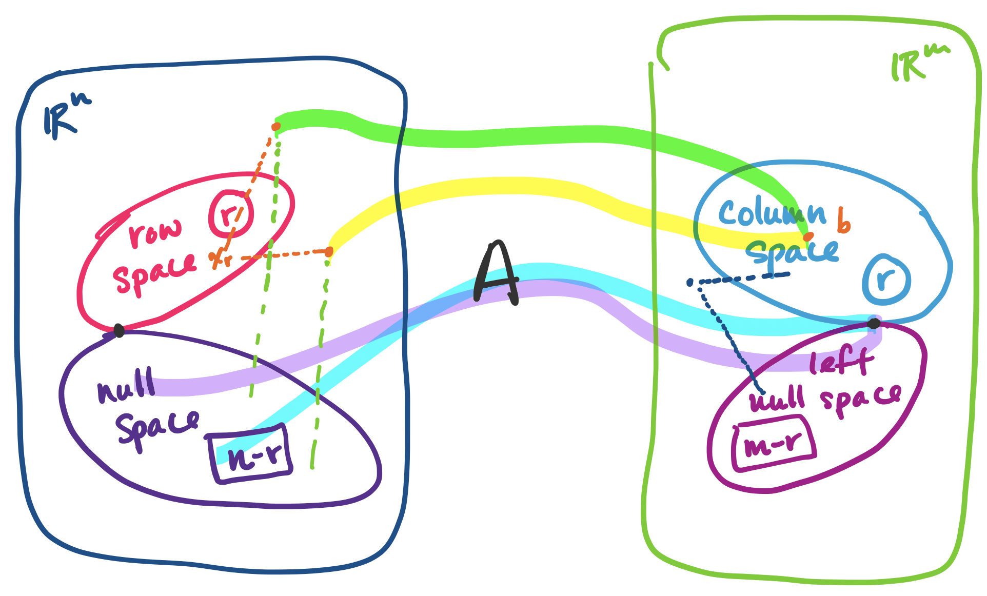
Put together, these facts about the dimensions of the fundamental subspaces forms the first part of what the textbook calls the "Fundamental Theorem of Linear Algebra".
Let $A$ be an $m \times n$ matrix of rank $r$.
This is only part 1, which connects the dimensions of the subspaces. This will allow us to work towards a bigger goal: being able to orient these subspaces with each other. We can begin to see something like this when we think about our complete solution.
Here is the same information in table form. If $A$ is an $m \times n$ matrix of rank $r$, then
| Name | Notation | Subspace of | Dimension |
|---|---|---|---|
| row space | $\mathbf C(A^T)$ | $\mathbb R^n$ | $r$ |
| column space | $\mathbf C(A)$ | $\mathbb R^m$ | $r$ |
| null space | $\mathbf N(A)$ | $\mathbb R^n$ | $n-r$ |
| left null space | $\mathbf N(A^T)$ | $\mathbb R^m$ | $m-r$ |
When discussing complete solutions to the equation $A \mathbf x = \mathbf b$, we came up with a way to describe them: find a particular solution $\mathbf x_p$ and add a vector from the null space of $A$. But $\mathbf x_p$ is actually a vector that's obtained via convenience, by setting the free variables to $0$.
One of the intriguing suggestions of the picture that we have is that a solution to $A \mathbf x = \mathbf b$ may be written instead as a vector $\mathbf x = \mathbf x_r + \mathbf x_n$—that is, every vector $\mathbf b$ in the column space of $A$ is associated with some vector $\mathbf x_r$ in the row space of $A$. Here, $\mathbf x_r$ is not necessarily $\mathbf x_p$, the particular solution. One can test this: take a particular solution and see if you can express it as a linear combination of rows. What this would say is that there's an even clearer partitioning of our data than we may have originally believed.
How this $\mathbf x_r$ interacts with vectors $\mathbf x_n$ in the nullspace is something we'll start talking about today. But there's more: this suggests that every vector in $\mathbb R^n$ can be expressed this way. And if this is true, we can say the same for vectors in $\mathbb R^m$: every vector in $\mathbb R^m$ can be written as a vector from the column space of $A$ together with a vector from the left null space of $A$. This is the beginnings of the strategy to being able to say something about how to deal with the question of $A \mathbf x = \mathbf b$ when there is no solution.
So far, we've dealt with vectors that are firmly located within our subspaces of interest—when we have solutions to $A \mathbf x = \mathbf b$. But what if the equation is unsolvable and $\mathbf b$ isn't in our column space?
From the perspective of data, this is a sample that lies outside of the space defined by some description of our dataset. What can we say about it? Well, we can determine which "point" is "closest" to it. However, this requires orienting our data and all of the subspaces we've been dealing with. After all, what does it mean for a vector to be "close" to some point of a vector space?
An important notion and tool for doing this orientation is the notion of orthogonality. Up until now, we've been dealing with sets of vectors like spanning sets and bases without thinking about their orientation—as long as they are independent and all point in a "new" direction, we've been happy. But a natural orientation is to have our basis vectors be orthogonal with each other—this property makes visualizing and computing with these objects much more convenient.
This is where a lot of the geometric notions we briefly introduced start coming into play. Recall the following properties and definitions.
Something that's often done in math is "lifting" a definition for a single item to a set of items. For instance, we have a definition for orthogonality of two vectors: they're at a 90° angle and their dot product is 0. We can then "lift" this definition to vector spaces.
Two subspaces $U$ and $V$ are orthogonal if every vector $\mathbf u$ in $U$ is orthogonal to every vector $\mathbf v$ in $V$. That is, $\mathbf u^T \mathbf v = 0$ for all $\mathbf u$ in $U$ and $\mathbf v$ in $V$.
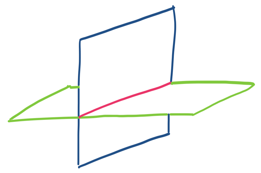
Consider the intersection of two planes at a 90° angle, like the walls of a room. These seem like they are orthogonal subspaces, but they aren't. The definition of orthogonality says that every vector in one subspace must be orthogonal to every vector in the other one. However, our two planes would intersect along a line The problem with this is that all the vectors at that intersection belong to both subspaces. This breaks our definition because it means there are a set of vectors that need to be orthogonal to themselves, which is impossible.
Note that by this definition, this means the only vector that can belong to two orthogonal subspaces is the zero vector. Our definition of orthogonality says that two vectors are orthogonal as long as their dot product is zero. The only vector for which that is true when taking a dot product with itself is $\mathbf 0$.
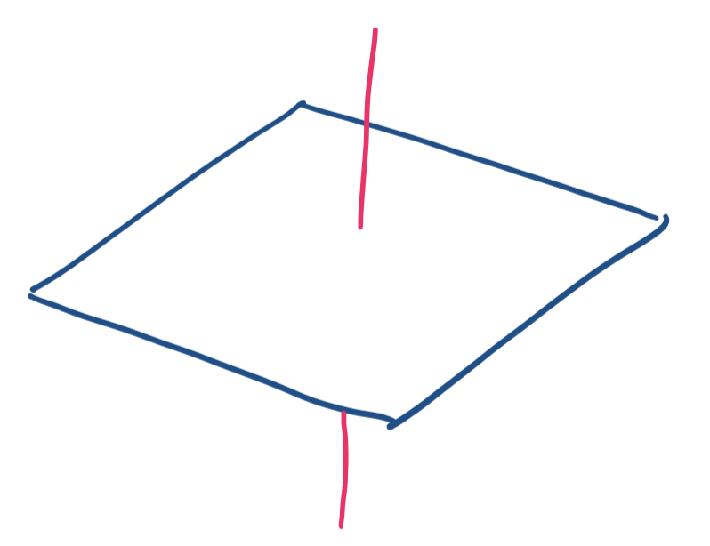
Consider the $x,y$-plane and the $z$ axis in $\mathbb R^3$. These are orthogonal subspaces: every vector on the $z$ axis is orthogonal to the $x,y$-plane and vice-versa.
These two examples suggest an interesting property: two subspaces can't be orthogonal if their dimensions together exceed the dimensions of the vector space they're in. In the first example, the planes were both 2-dimensional in a 3-dimensional space. In the second example, a line is 1-dimensional and the plane is 2-dimensional, which fits inside the 3-dimensional space.
With this, we can proceed to our big result.
Let $A$ be an $m \times n$ matrix. The null space of $A$ is orthogonal to the row space of $A$.
The null space is the set of all vectors $\mathbf x$ that satisfy $A \mathbf x = \mathbf 0$. So if $\mathbf a_1, \dots, \mathbf a_m$ are the rows of $A$ and $\mathbf x$ is a vector from the null space, we have that $\mathbf a_i^T \mathbf x = 0$ for every $i$. \[\begin{bmatrix} \rule[0.5ex]{3em}{0.5pt} & \mathbf a_1 & \rule[0.5ex]{3em}{0.5pt} \\ \rule[0.5ex]{3em}{0.5pt} & \mathbf a_2 & \rule[0.5ex]{3em}{0.5pt} \\ & \vdots & \\ \rule[0.5ex]{3em}{0.5pt} & \mathbf a_m & \rule[0.5ex]{3em}{0.5pt} \\ \end{bmatrix} \begin{bmatrix} \bigg\vert \\ \mathbf x \\ \bigg\vert \end{bmatrix} = \begin{bmatrix} \mathbf a_1^T \mathbf x \\ \mathbf a_2^T \mathbf x \\ \vdots \\ \mathbf a_m^T \mathbf x \end{bmatrix} = \begin{bmatrix} 0 \\ 0 \\ \vdots \\ 0 \end{bmatrix} \]
By definition, this means that every row vector of $A$ is orthogonal to $\mathbf x$. Since $\mathbf x$ is orthogonal to every row of $A$, it is orthogonal to any vector that is a linear combination of rows of $A$. So $\mathbf x$ is orthogonal to every vector in the row space of $A$. But $\mathbf x$ was any vector from the null space, so every vector in the null space of $A$ is orthogonal to every vector in the row space of $A$. So the null space is orthogonal to the row space.
Let $A = \begin{bmatrix} 1 & 3 & 1 \\ 1 & 9 & 3 \end{bmatrix}$. Then $\begin{bmatrix} 0 \\ -1 \\ 3 \end{bmatrix}$ is perpendicular to the rows of $A$. We see also that this means that it must be in the null space of $A$.
    >>> A = np.array([[1, 3, 1], [1, 9, 3]])
    >>> x = np.array([0, -1, 3])
    >>> A[0] @ x
    0
    >>> A[1] @ x
    0
    >>> A @ x
    array([0, 0])
There's another way of writing this by focusing on vectors.
Take a vector $\mathbf x$ from the null space of $A$. Now, take a vector from the row space of $A$. Recall that the row space of $A$ is the column space of $A^T$. So a vector from the row space can be written as a vector $A^T \mathbf y$ for some $\mathbf y$ in $\mathbb R^n$. That is, $A^T \mathbf y$ describes a linear combination of columns of $A^T$, but columns of $A^T$ are the rows of $A$. We get \[\mathbf x \cdot A^T \mathbf y = \mathbf x^T (A^T \mathbf y) = (\mathbf x^T A^T) \mathbf y = (A\mathbf x)^T \mathbf y = \mathbf 0^T \mathbf y = \mathbf 0 \cdot \mathbf y = 0.\] So $\mathbf x$ is a vector that is perpendicular to the vector $A^T \mathbf y$. So every vector in the null space of $A$ is perpendicular to every vector in the row space of $A$.
What is nice about this is that if we take $A$ and transpose it to $A^T$, we can do the exact same proof to get the following:
Let $A$ be an $m \times n$ matrix. The left null space of $A$ is orthogonal to the column space of $A$.
This quickly brought us to the second part of the Fundamental Theorem of Linear Algebra. First, we define the following notion.
Let $V$ be a subspace of a vector space $W$. The orthogonal complement $V^{\bot}$ of $V$ is the subspace of all vectors perpendicular to a vector in $V$. Furthermore, $\dim V + \dim V^{\bot} = \dim W$.
It is possible to have two very small orthogonal subspaces. For example, two lines can be orthogonal in $\mathbb R^6$. However, these would not be orthogonal complements. The definition says that two subspaces that are orthogonal complements will have dimensions that add to the full dimension of the vector space.
In fact, two spaces being orthogonal complements is a very strong relationship. Suppose we have two subspaces $V$ and $W$. If we know that a vector $\mathbf u$ is perpendicular to some basis for $V$, then we know it must belong to $W$.
Let $A$ be an $m \times n$ matrix. Then