Rank one products and rows
Let's go back to our factorization $A = CR$ and recall that one interpretation of this product is that each column of $R$ describes how to combine columns of $C$ to construct a column of $A$.
Notice that each row of $R$ is associated with a column of $C$. We can "decompose" our product in a different way.
Let $A = \begin{bmatrix} 1 & 2 & 4 \\ 3 & -2 & 4 \\ 2 & 3 & 7 \end{bmatrix} = \begin{bmatrix}1 & 2 \\ 3 & -2 \\ 2 & 3 \end{bmatrix} \begin{bmatrix} 1 & 0 & 2 \\ 0 & 1 & 1 \end{bmatrix}$. We have
\[\begin{bmatrix} 1 \\ 3 \\ 2 \end{bmatrix}\begin{bmatrix} 1 & 0 & 2 \end{bmatrix} + \begin{bmatrix} 2 \\ -2 \\ 3 \end{bmatrix} \begin{bmatrix} 0 & 1 & 1 \end{bmatrix} = \begin{bmatrix} 1 & 0 & 2 \\ 3 & 0 & 6 \\ 2 & 0 & 4 \end{bmatrix} + \begin{bmatrix} 0 & 2 & 2 \\ 0 &-2 & -2 \\ 0 & 3 & 3 \end{bmatrix} = \begin{bmatrix} 1 & 2 & 4 \\ 3 & -2 & 4 \\ 2 & 3 & 7 \end{bmatrix}.\]
What is the interpretation of this product? If the rank $r$ of a matrix is the number of independent columns it has, then it must have the same number of rows in $R$—one for each column. But our observation above was that each row of $R$ is associated to exactly one column of $C$. What we've done in the above example was separate each of these column/row pairs and turn them into products.
Each of these products has rank 1—the columns of each of these matrix products are clearly scalar multiples of each other. So this gives us another way to think about matrix products: as a sum of rank one products, or single column/row products. This view of the matrix product becomes very important near the end of the course as we think more about decomposition and approximation.
Finally, we'll see something that will be relevant in the upcoming section. What you notice here is that there is a very strong correspondence between the columns of $C$ and the rows of $R$. So a natural question to ask is: what about the rows of a matrix?
Again, let $A = \begin{bmatrix} 1 & 2 & 4 \\ 3 & -2 & 4 \\ 2 & 3 & 7 \end{bmatrix} = \begin{bmatrix}1 & 2 \\ 3 & -2 \\ 2 & 3 \end{bmatrix} \begin{bmatrix} 1 & 0 & 2 \\ 0 & 1 & 1 \end{bmatrix}$. We constructed the first row of $A$ by looking at the first column of $R$: take 1 of column 1 of $C$ and take 0 of column 2 of $C$.
But we can try doing this with rows of $R$. The first row of $C$ says to take 1 of row 1 of $R$ and 2 of row 2 of $R$. This gives us
\[\begin{bmatrix} 1 & 0 & 2 \end{bmatrix} + \begin{bmatrix} 0 & 2 & 2 \end{bmatrix} = \begin{bmatrix} 1 & 2 & 4 \end{bmatrix}.\]
So in fact, we can interpret $A = CR$ in terms of rows as well: rows of $C$ tell us how to combine rows of $R$ to construct rows of $A$.
This tells us some very important things:
- We can view $CR$ as the rows of $R$ describing how to combine columns of $C$.
- We can view $CR$ as the columns of $C$ describing how to combine rows of $R$.
- The order of matrix multiplication matters—notice that whether we're talking about combinations of rows or columns depends on the relative position of $C$ and $R$ with each other.
Matrices as functions
There is one more point to discuss about matrices and matrix products. Let's think back to the view of matrices as functions that transform vectors into other vectors. Just like we did matrix-vector products, we can extend this idea to matrices as functions that transform matrices into other matrices. This leads us to a number of interesting matrices.
The identity matrix $I$ is the matrix such that $AI = A$ and $IA = A$.
Let $A = \begin{bmatrix} 2 & 4 \\ 3 & 4 \end{bmatrix}$ and observe that
\[AI = \begin{bmatrix} A \begin{bmatrix} 1 \\ 0 \end{bmatrix} & A \begin{bmatrix} 0 \\ 1 \end{bmatrix} \end{bmatrix} = \begin{bmatrix} 1 \begin{bmatrix} 2 \\ 3 \end{bmatrix} + 0 \begin{bmatrix} 4 \\ 4 \end{bmatrix} & 0 \begin{bmatrix} 2 \\ 3 \end{bmatrix} + 1 \begin{bmatrix} 4 \\ 4 \end{bmatrix} \end{bmatrix} = \begin{bmatrix} 2 & 4 \\ 3 & 4 \end{bmatrix} = A.\]
In other words, we have a matrix that encodes the linear combination that "selects" the corresponding column in each position. Similarly, we have
\[IA = \begin{bmatrix} I \begin{bmatrix} 2 \\ 3 \end{bmatrix} & I \begin{bmatrix} 4 \\ 4 \end{bmatrix} \end{bmatrix} = \begin{bmatrix} 2 \begin{bmatrix} 1 \\ 0 \end{bmatrix} + 3 \begin{bmatrix} 0 \\ 1 \end{bmatrix} & 4 \begin{bmatrix} 1 \\ 0 \end{bmatrix} + 4 \begin{bmatrix} 0 \\ 1 \end{bmatrix} \end{bmatrix} = \begin{bmatrix} 2 & 4 \\ 3 & 4 \end{bmatrix} = A.\]
The effect of this is the same, but the interpretation can be slightly different.
The identity matrix is a square matrix with ones along its diagonal and zeroes everywhere else. Although we call it the identity matrix, there is really an identity matrix for each size $n$. An interesting question you can work out on your own is: show that there's only one identity matrix of each size $n$.
Generally speaking, this form of a matrix is nice enough to be of note.
A diagonal matrix is a matrix with nonzero entries only along its diagonal and zeroes elsewhere.
Suppose we have a $2 \times 2$ matrix $A = \begin{bmatrix} 2 & 4 \\ 3 & 4 \end{bmatrix}$ and consider the transformation where we simply exchange the columns so we end up with the matrix $B = \begin{bmatrix} 4 & 2 \\ 4 & 3 \end{bmatrix}$. This strange action is also just a bunch of linear combinations put together. Let $\mathbf a_1$ and $\mathbf a_2$ denote the columns of $A$. Then the first column of $B$ is just $0 \cdot \mathbf a_1 + 1 \cdot \mathbf a_2$ and the second column of $B$ is $1 \cdot \mathbf a_1 + 0 \cdot \mathbf a_2$. Putting these two linear combinations together gives us the matrix $\begin{bmatrix} 0 & 1 \\ 1 & 0 \end{bmatrix}$.
We can try the same thing out with three columns. For instance, what if we want to swap columns 1 and 3, while keeping column 2 in place? We reason in the same way: we think about how to construct
- the first column: zero out the other two columns and take the third,
- the second column: zero out the other two columns and take the second,
- the third column: zero out the other two colums and take the third.
From this, we arrive at the matrix $\begin{bmatrix} 0 & 0 & 1 \\ 0 & 1 & 0 \\ 1 & 0 & 0 \end{bmatrix}$.
This is maybe a bit strange, that we can view matrices both as data and as a function that transforms vectors. But this is actually a shade of a central idea in computer science: that data and functions are really the same thing. There are a few ways you may have encountered this idea already:
- Functions in Python (and functional programming languages in general) can be treated as data that you can assign to variables and pass around as inputs for other functions.
- The programs that you write are functions in the sense that they compute something, but they are also data because they are literally text. This text gets passed as data into the Python interpreter (a function), which produces some output: Python bytecode, which is itself data (ones and zeros are just a binary string or number) and a function (an executable program).
The idea of the matrix as a function is also the perspective that machine learning takes. Formally, the problem that machine learning tries to solve is learning a function. That is, given some kind of input (exemplar inputs, some description of the desired output, etc.) the algorithm tries to "learn" the function and the outcome is a function that tries to behave like the function that the algorithm attempts to learn. Such a function would be an approximation of the true function. Then from the linear algebra perspective, we have a matrix that is an approximation of the "true" matrix.
Linear Equations
Recall that our primary goal here is to learn something about a given matrix $A$: what is its rank, which columns are independent, and so on. In order to do this, we need to study the classical problem that linear algebra tries to solve: finding solutions to systems of linear equations.
Suppose we have a system of equations
\begin{align*}
2x + 3y &= 7 \\
4x - 5y &= 11 \\
\end{align*}
We can write this as a matrix $A$ and vectors $\mathbf x$ and $\mathbf b$,
\[\begin{bmatrix} 2 & 3 \\ 4 & -5 \end{bmatrix} \begin{bmatrix}x \\ y \end{bmatrix} = \begin{bmatrix}7 \\ 11 \end{bmatrix}.\]
We see here that we can reformulate this problem in terms of linear algebra: given matrix $A$ and vector $\mathbf b$, find all vectors $\mathbf x$ such that
\[A \mathbf x = \mathbf b.\]
You probably don't even need linear algebra to solve such problems, given enough time to do it. Perhaps unsurprisingly, thinking about this problem through the lens of linear algebra will give us more insights into the properties of matrices and vectors.
We can think about this problem in two ways. First, in the way that you've probably seen, what we want to do is find real number solutions $x$ and $y$ that satisfy our equations. This is the "dot product" view of the matrix-vector product $A \mathbf x$.
Secondly, in the way that you're not used to, what we want to do is find a vector $\mathbf x$ that satisfies our equation. If we recall what matrix-vector products mean, what this is really asking is to find how to combine columns of $A$ to construct the vector $\mathbf b$. That is, can $\mathbf b$ be written as a linear combination of columns of $A$?
Typically, we would like one solution (this was likely the running assumption in these kinds of problems you've seen in the past), but that's not the only possibility. We will also be considering the cases where there could also be no solution for this system, or there could be infinitely many solutions. Each of these situations translates into something about the columns of our matrix $A$.
- If there's exactly one solution, then we know that the columns of $A$ must be linearly independent. Why? We'll convince ourselves in a bit, but let's move on.
- However, if $A \mathbf x = \mathbf b$ doesn't have any solutions, we can say something about that: there are no linear combinations of columns of $A$ that give us $\mathbf b$!
- But what if there are infinitely many solutions? This suggests that the columns of $A$ are linearly dependent!
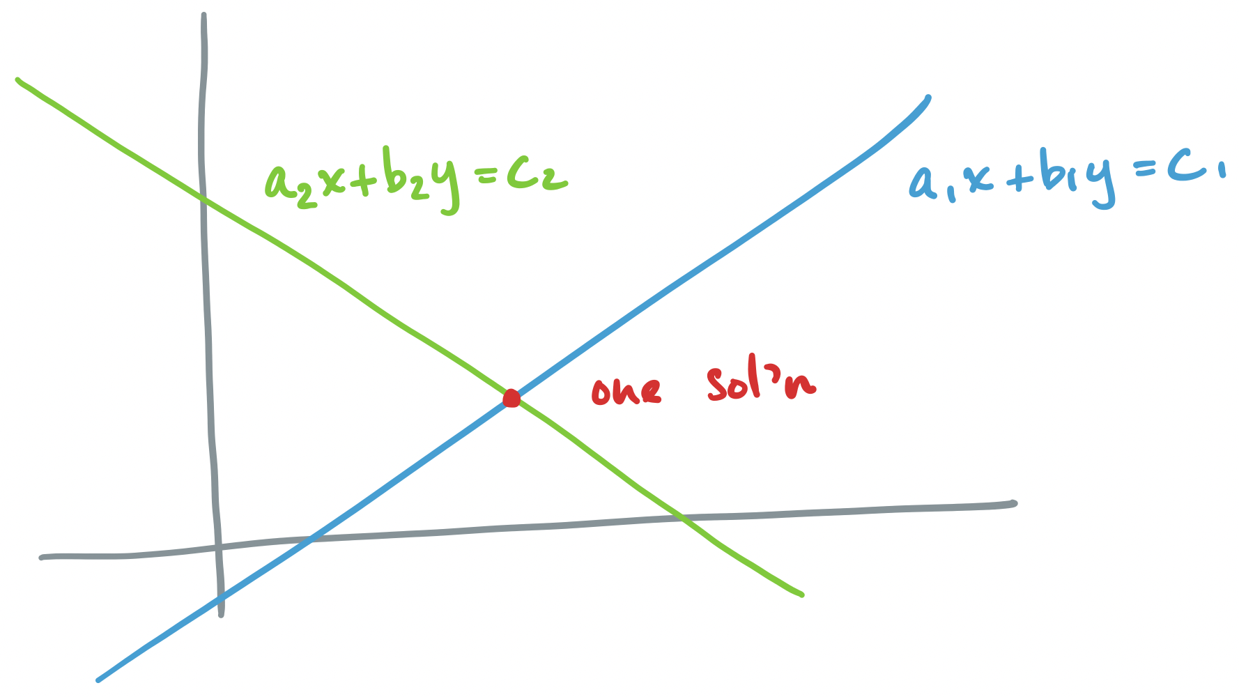
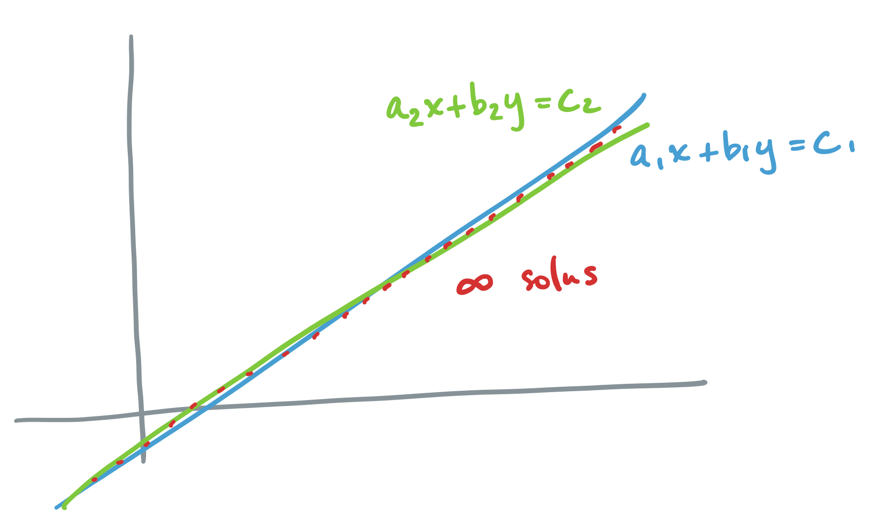
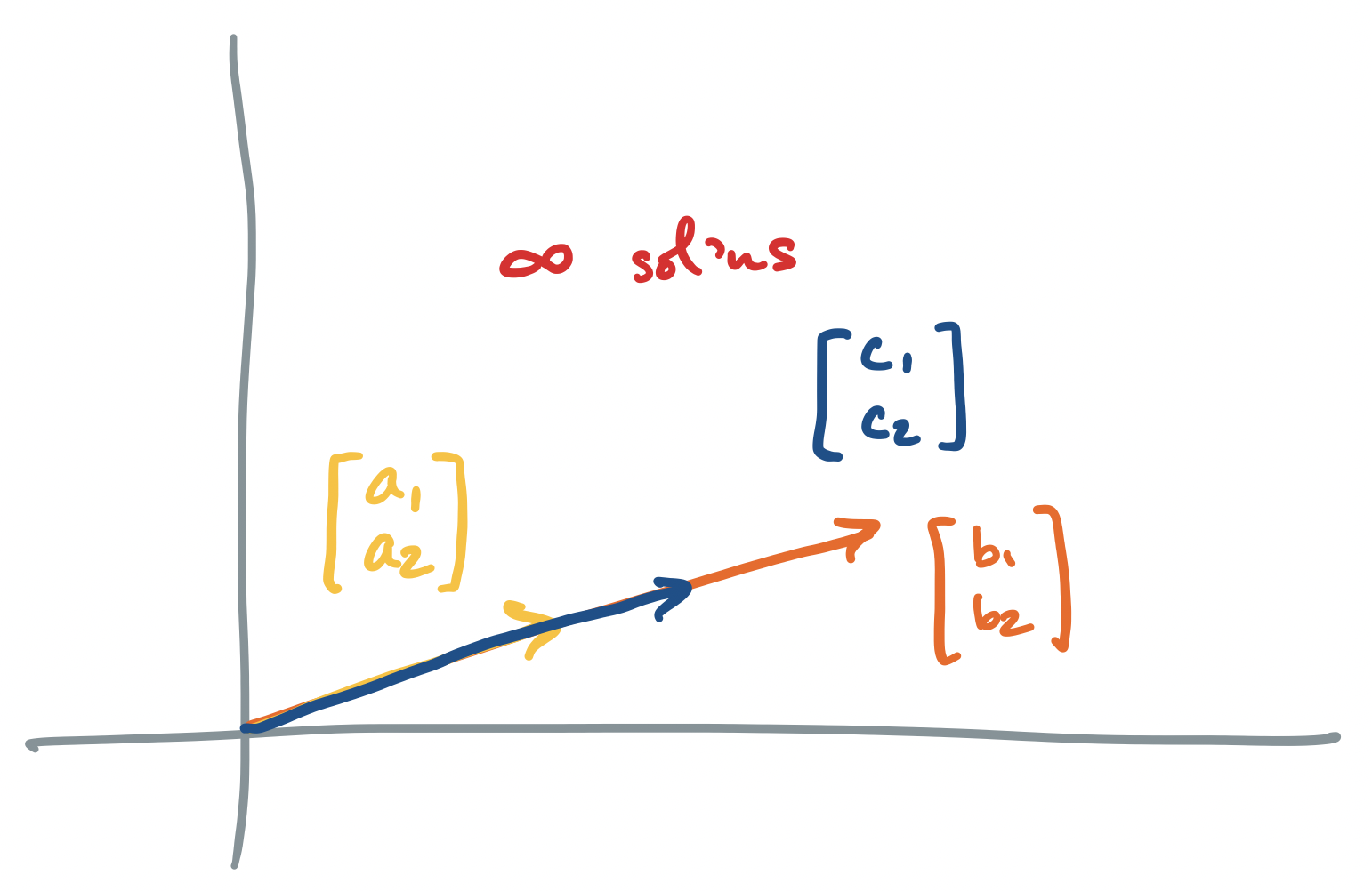
Each of these scenarios can be depicted pictorally, either through the traditional view of geometry (what Strang calls the "row picture"), where equations are drawn as lines or planes on the Euclidean plane, or by the view of linear combinations that we described above (called the "column picture")
Let's go through each scenario described above, for the system $A \mathbf x = \mathbf b$ where $A = \begin{bmatrix} a_1 & b_1 \\ a_2 & b_2 \end{bmatrix}$ and $\mathbf b = \begin{bmatrix} c_1 \\ c_2 \end{bmatrix}$.
-
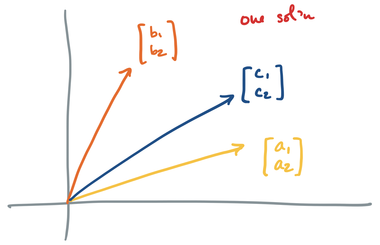
If $A\mathbf x = \mathbf b$ has exactly one solution, the row picture says that there is exactly one point at which all of our equations intersect. The corresponding column picture is that of linearly independent vectors for which there exists one linear combination to describe $\mathbf b$.
-
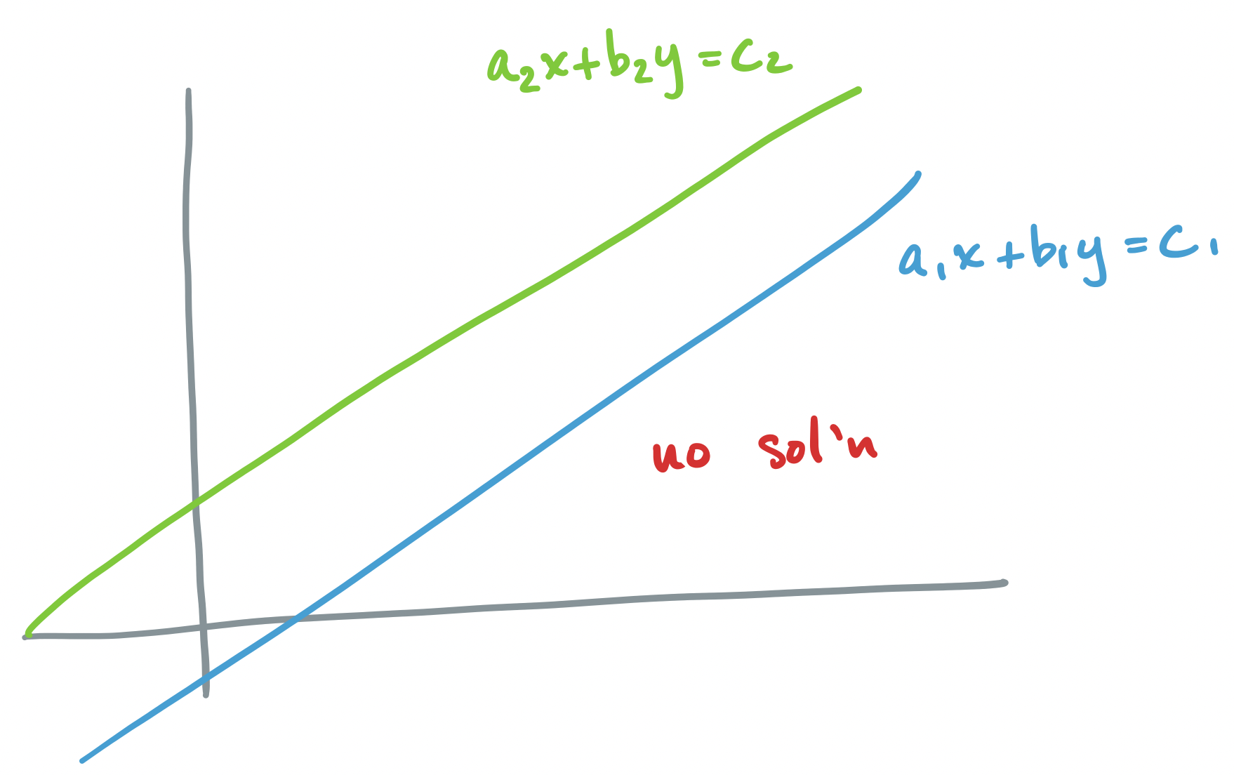
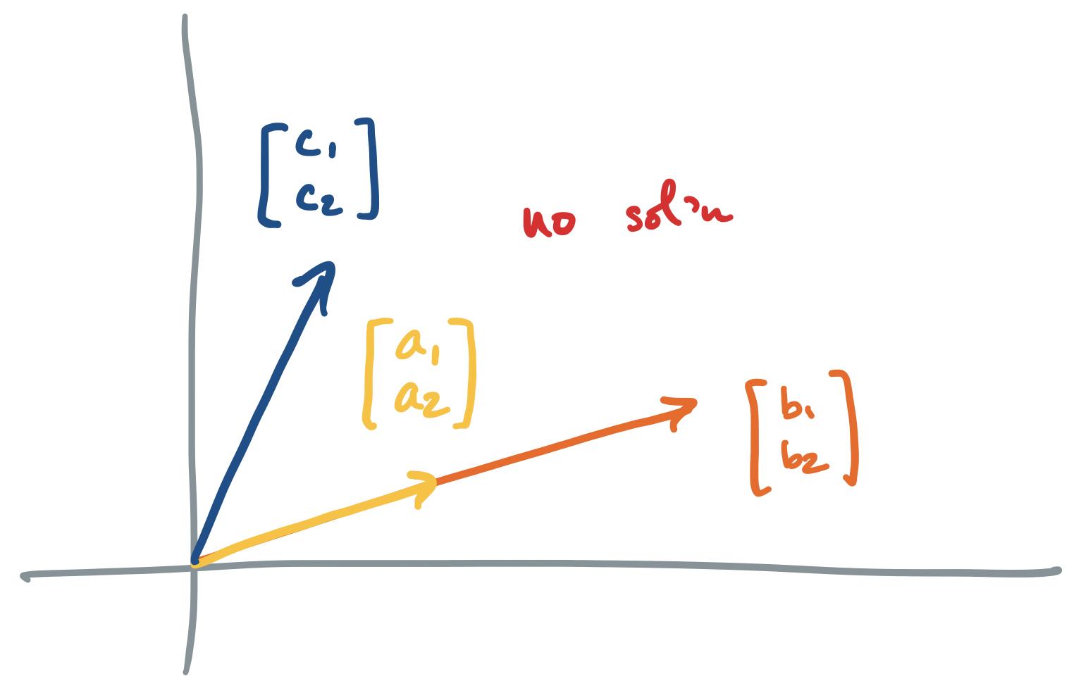
If $A \mathbf x = \mathbf b$ has no solution, we said above that the column picture says that there are no linear combinations of our column vectors that produces $\mathbf b$. The traditional row picture describes two objects (lines, planes, etc) which do not intersect.
-
If $A \mathbf x = \mathbf b$ has infinitely many solutions, we said above that we have linearly dependent columns. So the column picture says that we have infinitely many ways to combine our column vectors to produce $\mathbf b$. The row picture describes two objects (lines, planes, etc) which intersect along at least a line, but maybe even a plane or more in higher dimensions. Since lines are infinitely long, there are infinitely many intersection points.
We're already familiar with the idea of linear independence as being about for some collection of vectors, whether any of the vectors can be written as a linear combination of the others. While this definition is intuitive, it's actually a bit cumbersome to use, so here's another definition that captures the same idea.
The vectors $\mathbf v_1, \dots, \mathbf v_n$ are said to be linearly independent if and only if the only linear combination $a_1 \mathbf v_1 + \cdots + a_n \mathbf v_n = \mathbf 0$ is $a_1 = \cdots a_n = 0$.
Why is this definition the same as our more intuitive definition? Consider the situation in which we have vectors that are not independent. So $a_1 \mathbf v_1 + a_2 \mathbf v_2 = \mathbf v_3$. If we rearrange this equation, we get $a_1 \mathbf v_1 + a_2 \mathbf v_2 - \mathbf v_3 = \mathbf 0$. This is a linear combination of the vectors that produces $\mathbf 0$ but the scalars aren't all 0.
This helps us understand why having linearly dependent columns can give us infinitely many solutions for an equation $A \mathbf x = \mathbf b$. Suppose $A$ has linearly dependent columns, say $\mathbf u$ and $\mathbf v$. Then I have $\mathbf u = c \mathbf v$ for some scalar $c$. Well, this gives us $\mathbf u - c\mathbf v = \mathbf 0$, which means that there exists a vector $\mathbf y$, which encodes this linear combination such that $A\mathbf y = \mathbf 0$ and $\mathbf y \neq \mathbf 0$. Then I can take another scalar $k$ and get (infinitely) more combinations of these vectors that give me $k (A \mathbf y) = A(k \mathbf y) = \mathbf 0$.
Now, notice that $A \mathbf x = A \mathbf x + \mathbf 0 = \mathbf b + \mathbf 0 = \mathbf b$. If I have linearly dependent columns, I have infinitely many ways to get $\mathbf 0 = A(k\mathbf y)$, which means that
\[\mathbf b = A \mathbf x = A \mathbf x + \mathbf 0 = A \mathbf x + A(k \mathbf y) = A(\mathbf x + k \mathbf y),\]
and therefore $\mathbf x + k \mathbf y$ is a solution for all scalars $k$. On the other hand, if I have linearly independent columns, $\mathbf 0$ is the only linear combination of columns of $A$ that gets me $\mathbf 0$.