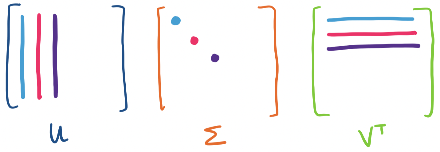
So far, we've discussed SVD largely in terms of its matrix composition $U \Sigma V^T$. However, the other representation of SVD, that $A = \sigma_1 \mathbf u_1 \mathbf v_1^T + \cdots + \sigma_r \mathbf u_r \mathbf v_r^T$ is the main tool that we'll start using.
The reduced SVD actually immediately gives us an application: compression. Consider an $m \times n$ matrix. Such a matrix obviously has $mn$ values. But do we need to store all of those values? If the rank of the matrix is $r$, then the reduced SVD gives us a way to store those values using only $mr + nr + r = r(m+n+1)$ values—this is much smaller than $m \times n$ if $r$, the rank of the matrix, is much smaller. And this is without losing any information at all—we'll see soon that if we're okay with losing some information, SVD gives us a principled way to do lossy compression.
The main idea behind data science and machine learning applications is that we often have data that is too large and too complicated to work with. So far, we have invested a lot of time into understanding how to break down matrices so that we can work with simpler pieces: linearly independent vectors and bases, subspaces, orthogonal and orthonormal bases, least squares approximations, diagonalization.
What we're really looking for is a low-dimensional approximation of our data. In other words, we want a simpler version of our data that still retains the essential characteristics and structures in our original dataset, but in a more tractable form.
One of the main complicating factors of this is the fact that there are too many dimensions to the data. This is an issue for a number of reasons. One obvious one is that it makes the data computationally expensive to process. Another reason is that high-dimensional data is often more sparse—there are more dimensions/ways for data to be "different" from each other, making identifying commonalities like clusters more difficult. And yet, it's observed that real data tends to lie along low-dimensional subspaces.
The SVD gives us a way to extract these low dimensional subspaces. The idea is simple: we can construct an approximation for $A$ of rank $k$ by using the top $k$ singular vectors.
Let $A = \sigma_1 \mathbf u_1 \mathbf v_1^T + \cdots + \sigma_r \mathbf u_r \mathbf v_r^T$ with $\sigma_1 \geq \cdots \geq \sigma_r \gt 0$. We define the rank $k$ approximation of $A$ to be the matrix \[A_k = \sigma_1 \mathbf u_1 \mathbf v_1^T + \cdots + \sigma_k \mathbf u_k \mathbf v_k^T.\]
The idea is simple: if we view the SVD as a weighted sum of rank 1 matrices weighted by the singular values, then to get a rank $k$ approximation, we take the rank 1 matrices with the largest weight—those associated with the first $k$ singular values.
The obvious question to ask is how good of an approximation this is. We have the following result due to Eckart and Young in 1936.
Let $A$ be a matrix and let $A_k$ be the rank $k$ approximation obtained via the SVD. If $B$ is a matrix of rank $k$, then $\|A - A_k\| \leq \|A-B\|$.
Eckart and Young were both here, at the University of Chicago (Eckart as a professor in Physics and Young as a grad student), when they published their proof of this result.
What this says is that the rank $k$ matrix obtained by summing the $k$ largest rank 1 matrices based on singular values is the best rank $k$ approximation of $A$. That is, among all matrices of rank $k$, $A_k$ is the closest to $A$. That is, the SVD gives us the best possible rank $k$ approximation of $A$.
There's just one piece missing from this: what does it mean for two matrices to be "close"? The theorem tells us, it's when the "distance" between the two is small, as measured by $\|A-B\|$. This looks like the "length" of the matrix, but what does a matrix length even mean?
The technical term for what we've been calling the "length" of a vector is the norm of the vector. Norms are functions that obey certain rules to give us a notion of "closeness" or "similarity" between two objects. Here's a technical definition of the rules involved.
A norm on a vector space $V$ is a function $\|\cdot\|: V \to \mathbb R$, which assigns to a vector $\mathbf x$ a scalar $\|\mathbf x\|$ such that for all scalars $c$ and vectors $\mathbf x, \mathbf y$,
| Formal condition | Informal meaning |
|---|---|
| $\|\mathbf x\| \geq 0$ | The norm is nonnegative |
| $\|\mathbf x\| = 0$ if and only if $\mathbf x = \mathbf 0$ | A vector has norm 0 if and only if it is the zero vector |
| $\|c\mathbf x\| = |c| \|\mathbf x\|$ | Norms are scaled by scalars |
| $\|\mathbf x + \mathbf y\| \leq \|\mathbf x\| + \|\mathbf y\|$ | The norm obeys the triangle inequality: the length of one side ($\mathbf x + \mathbf y$) can't be longer than the sum of the other two sides |
| $\|\mathbf u^T \mathbf v\| \leq \|\mathbf u\| \|\mathbf v\|$ | The norm obeys the Schwarz inequality: the norm of the (inner) product of the vectors can't exceed the product of the norms of the vectors |
Notice that this defines a norm over a vector space—recall that matrices are also "vectors" with respect to some vector space. So any matrix norms we define will use the same rules, which is very convenient. Just like the vector space rules, you don't really need to memorize these, since the idea behind these rules is that a norm should in some sense look and feel like what you'd expect a norm to do: give some notion of "length" or "size" to the object.
This means that objects can have more than one norm defined for them. This means that we've already been implicitly dealing with a choice of a vector norm that we made without thinking too deeply. In fact, our vector length is really the Euclidean norm, also called the $\ell_2$ norm.
What other vector norms are there? One such norm is the taxicab norm
The $\ell_1$ norm, informally called the taxicab norm or Manhattan norm, is defined for a vector $\mathbf v = \begin{bmatrix} v_1 \\ \vdots \\ v_n \end{bmatrix}$ in $\mathbb R^n$ by $\|\mathbf v\|_1 = |v_1| + \cdots + |v_n|$.
Why should we want different notions of length? Though these notions are defined mathematically, they appear in the real world as well. Suppose you're at State and Madison ($(0,0)$ on Chicago's grid) and you need to head over to the Thompson Center (Clark and Randolph) to renew your driver's license. How long does it take for you to get there?
The answer that you would expect is that it's two blocks north then two blocks west. Since a block is an eigth of a mile (or 200 m), this is half a mile (or 800 m). This answer is an example of the $\ell_1$ norm. The $\ell_2$ norm, the Euclidean distance would draw a straight line from State and Madison to Clark and Randolph and give us a distance of $\frac{\sqrt 2}{4}$ miles (or $400\sqrt 2$ m). Which is "correct"? It depends on your application!
Here's a more mathematical use for this norm. Recall that stochastic matrices are those whose column entries add to 1. In fact, this is really just the condition that the $\ell_1$ norm of the columns is 1. Notice that such vectors would not have unit length under the Euclidean norm.
We give three norms for a matrix $A$:
These are the strict definitions of the norms. However, each one of them is connected to the singular values of $A$.
Let $A$ be a matrix with nonzero singular values $\sigma_1 \geq \dots \geq \sigma_r \gt 0$. Then
These are probably the definitions of the norms you want to keep in mind. One interesting consequence of this is that it tells us that singular values themselves obey the rules of norms.
Consider two matrices $A$ and $B$ with first singular values $\alpha_1$ and $\beta_1$, respectively. Then the first singular value for $A+B$ cannot be any larger than $\alpha_1 + \beta_1$. Why? If this were the case, then $\|A+B\|_2 \gt \|A\|_2 + \|B\|_2$.
In summary,
| Name | Notation | Formal definition | Relationship to singular values |
|---|---|---|---|
| spectral | $\|A\|_2$ | maximum of ratio $\frac{\|A\mathbf x\|}{\|\mathbf x\|}$ over all vectors $\mathbf x$ (i.e. the longest a vector can get when multiplied by $A$) | $\sigma_1$, the largest singular value of $A$ |
| Frobenius | $\|A\|_F$ | square root of sum of squares of entries of $A$ | square root of sum of squares of singular values of $A$ |
| nuclear | $\|A\|_N$ | sum of diagonal entries (i.e. trace) of matrix square root of $A^TA$ (i.e. matrix inner product) | sum of singular values of $A$ |
Why do we have three different matrix norms? In fact, there are many more matrix (and vector) norms out there, each with their own meanings and applications. Each norm captures something different about the matrix $A$ as a transformation.
However, we mention these ones in particular because these norms all apply to the Eckart–Young theorem. This result is due to Mirsky in 1960: Eckart–Young holds for any norm that depends only on singular values. So for any of the matrix norms we mentioned, it will always be the case that $\|A - A_k\| \leq \|A - B\|$ for all rank $k$ matrices $B$.
Principal Component Analysis is a technique that has its origins in statistics. This is not a statistics class. Instead, like linear regression, we'll view it structurally. In this view, the basic idea of PCA is to find a low-dimensional representation or description (i.e. some subspace) for some data that we have. Obviously, we would like such a description to have minimal error. For a dataset $\mathbf a_1, \dots, \mathbf a_n$, this is done by minimizing the distances of all $\mathbf a_i$ to such a subspace. The goal of PCA is to find an orthonormal basis $\mathbf q_1, \dots, \mathbf q_k$ for this "best $k$-dimensional subspace of fit".
This sounds suspiciously similar to the least squares linear regression we were doing a few weeks ago. It's not entirely off-base: linear regression is also trying to find a low-dimensional subspace of best fit. But there's a subtle difference in what the two methods are trying to accomplish. Suppose we have the following dataset.
| $t$ | $b$ |
|---|---|
| -15 | 7 |
| -2 | -9 |
| 4 | -15 |
| 9 | -10 |
First, let's think about what such a basis would look like with respect to our dataset. What we want to do is to minimize all of the distances from every $\mathbf a_i$ to their projections onto our subspace. The orthogonality of our basis is helpful in this case: this means all we need is to consider the projections onto each dimension, one at a time, because they don't "interfere" with each other.
Again, we note that this differs from least squares regressions, which seeks to compute $\mathbf x$ so that it minimizes $\|A \mathbf x - \mathbf b\|^2$. Instead, we try to find a basis vector that minimizes $\|\mathbf e\|^2$, the error term or in this case, the distance between $\mathbf a_i$ and its projection onto the basis vector. The difference is captured below.
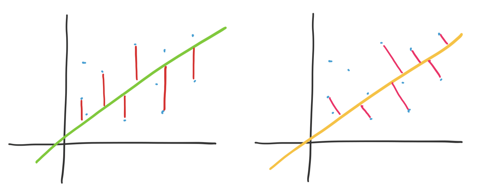
On the left is the view of least squares: minimizing the "vertical" distance to the line of best fit. On the right is view of principal component analysis: minimizing the distance to the line of best fit—this is perpendicular rather than vertical. What's the difference? In the case of regression, only the distance concerning the target variable (i.e. the vertical distance) matters, while in PCA, the distance over the entire space matters.
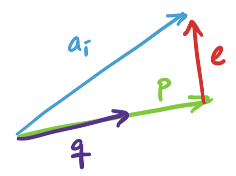
Since we can break up our search for $k$ basis vectors into one dimension at a time, we can consider the one dimensional case, where we project $\mathbf a_i$ onto some unit vector $\mathbf q$. This projection is $\mathbf p = \mathbf q \mathbf q^T \mathbf a_i$. We have ourselves a right triangle again and we see that the lengths work out so that we have
\[\|\mathbf a_i\|^2 = \|\mathbf q \mathbf q^T \mathbf a_i\|^2 + \|\mathbf e\|^2.\]
Again, the goal is to minimize the distance $\|\mathbf e\|^2$. Since $\mathbf a_i$ is fixed, our only choice is to find $\mathbf q$ so that $\|\mathbf q \mathbf q^T \mathbf a_i\|^2$ is as large as possible. What exactly is this quantity? Recall that $\mathbf q^T \mathbf a_i$ is the dot product $\mathbf q \cdot \mathbf a_i$. This means we can view $\mathbf q \mathbf q^T \mathbf a_i$ as $(\mathbf q \cdot \mathbf a_i)\mathbf q$, a scalar multiple of $\mathbf q$. Since $\|\mathbf q\| = 1$, the length of the resulting projection is exactly $\mathbf q \cdot \mathbf a_i$, making $\|\mathbf p\| = (\mathbf q \cdot \mathbf a_i)^2$.
Now, suppose we have all of our $\mathbf a_i$'s in a single matrix $A$. To compute $(\mathbf q \cdot \mathbf a_i)^2$ for all of these at the same time, we have \[\sum_{i=1}^n (\mathbf a_i \cdot \mathbf q)^2 = (A\mathbf q)^T (A \mathbf q) = \mathbf q^T A^T A \mathbf q.\] Again, recall that $A$, which contains our dataset is fixed, which must mean that what we need to do is try to find $\mathbf q$ that maximizes the quantity above. This matters because we see a familiar friend that will help us accomplish this: $A^TA$.
We've just seen $A^TA$: it's $V \Sigma^2 V^T$ from the SVD. Let's consider what happens when we take $\mathbf q^T V \Sigma^2 V^T \mathbf q$. Since $V$ is orthogonal, the length of $\mathbf q$ doesn't get changed by $V$. That is $\|V \mathbf q\| = \|\mathbf q\|$. However, $\Sigma^2$ does change its length: it "stretches" the vector according to its linear combination by $V$. After this stretching, its length doesn't change again since $\|\mathbf q\| = 1$.
This suggests we can view unit vectors undergoing a transformation through $A^TA$ as having length that "averages" the eigenvalues $\sigma_i^2$. So it seems that to maximize this value, we need to maximize the involvement of the eigenvector with the largest eigenvalue. By convention, this eigenvector is $\mathbf v_1$, which has eigenvalue $\sigma_1^2$.
The result is that the vector $\mathbf q$ that maximizes $\mathbf q^T A^TA \mathbf q$ is $\mathbf v_1$, the first singular vector. What we get is \[\|A \mathbf v_1\|^2 = \mathbf v_1^T (A^TA \mathbf v_1) = \mathbf v_1^T (\sigma_1^2 \mathbf v_1) = \sigma_1^2 (\mathbf v_1^T \mathbf v_1) = \sigma_1^2.\]
The claim is that any other unit vector $\mathbf q$ gives us $\mathbf q^T A^TA \mathbf q \leq \sigma_1^2$. Notice that this leads us directly to the spectral norm. If we want to generalize this argument for any vector $\mathbf x$, we need to consider the length of $\mathbf x$. This is easy: just normalize it. So we have \[\frac{\mathbf x^T}{\|\mathbf x\|} A^T A \frac{\mathbf x}{\|\mathbf x\|} = \frac{\mathbf x^T A^T A \mathbf x}{\|x\|^2} = \frac{\|A\mathbf x\|^2}{\|\mathbf x\|^2} \leq \sigma_1^2,\] which gives us $\frac{\|A \mathbf x\|}{\|\mathbf x\|} \leq \sigma_1$ for all nonzero vectors $\mathbf x$.
Since we assume we want an orthonormal basis (and this guarantees that we will get one by the diagonalization of $A^TA$), we simply repeat this process for each successive dimension: the next vector that maximizes the next direction will be $\mathbf v_2$, and so on. What we find is exactly what we want: the principal components are the vectors associated with the largest singular vectors.
So we've seen that SVD gives us PCA almost for free. The other side of the coin is that PCA confirms that SVD does indeed give us the best rank $k$ approximation of $A$, by convincing us that the principal components coincide with the singular vectors associated with the largest singular values.
Let's think back to the beginning of the quarter. We had this notion of vectors as objects that could be added together and scaled. These represent objects or data. Since they're finite dimensional, we can focus our attention on $\mathbb R^n$ (things would be a bit different if we considered infinite-dimensional vector spaces).
We are concerned with collections of data, which means we need to work with collections of vectors. Such objects are matrices. Like vectors, we can combine matrices in certain ways, the most significant of which was via matrix multiplication. Matrix multiplication was already enough to lead to our first example: the recommendation system. This was the setup in which our matrix $A$ contained ratings of products by users, with each column representing a user profile and each row representing a product.
At the time, we had the following observations.
All of this was achieved simply through understanding the mechanism of matrix multiplication. This led to the following questions:
These are questions that involve ideas about linear independence, vector spaces, and bases. Over the course of the course, we got some answers.
But there's a problem:
The singular value decomposition and low-rank approximations close the loop on these questions. SVD combines everything that we've done in the course to give us a way out:
Notice the work required to get here:
These are the basic ingredients for working with matrices and linear data. And these are the basic ideas that machine learning algorithms and data analysis techniques exploit to uncover the latent structures laying hidden inside data. Obviously, there are many more sophsiticated approaches and techniques out there, but they all build on a basic understanding of these fundamental pieces.
We'll lean once more on the idea of the SVD giving us a weighted sum of rank 1 matrices to discuss compression. As mentioned before, the SVD gives us a way to losslessly compress a matrix. By lossless, we mean that the original matrix can be reconstructed perfectly.
However, lossless compression is not viable or necessary in many cases. Much of the digital media we use is compressed lossily: the most widely used image, audio, and video compression algorithms are lossy. The idea behind lossy compression is that exact replication is not necessary because much of the detail that is lost is either undetectable or is just noise.
In some sense, this ties back into the idea of information theory viewed through the lens of machine learning. Machine learning is all about mechanistically trying to find regularities and structure in data. The goal of this is to be able to acquire a simpler description. Such a description is compression in information theoretic terms.
Section 7.2 of the textbook discusses a direct application of this idea: image compression. The idea is that an image is just a grid of pixels. Of course, a matrix is just a grid, so it makes perfect sense to represent an image as a matrix. We can then apply linear algebra tools to process images.
The following images are of the same photo of a pile of Blåhaj at IKEA Shibuya. The original is at the bottom right. From the top left, we have the rank 1, 10, 20, 100, and 200 approximations obtained via SVD (using this convenient online demo).

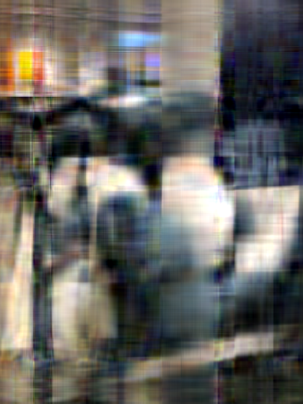
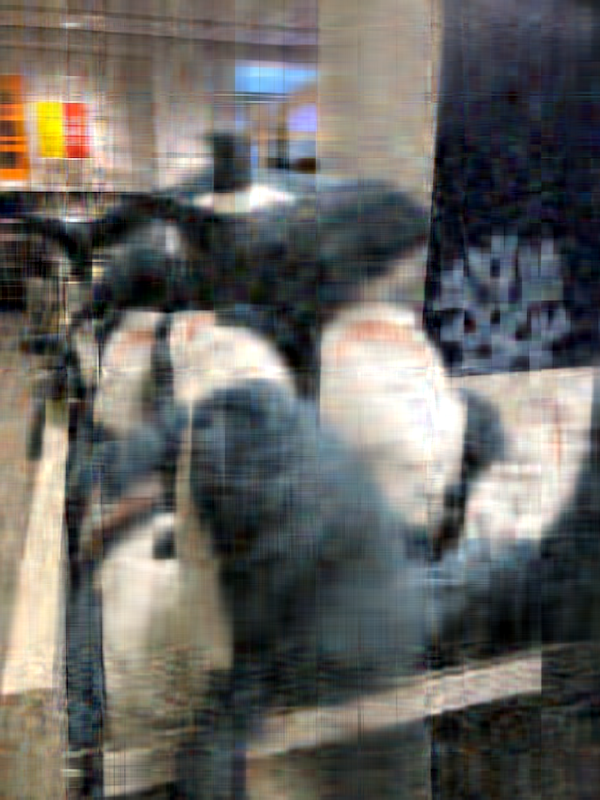


It's hard to see at the current size on this page, but if you view the images at their actual size, you'll see that there is still a slight but noticeable difference between the rank 100 approximation and the rank 200 approximation, but the rank 200 approximation is virtually indistinguishable from the original.
One can compute approximately how good this compression is based on the sizes of the matrices. The original photo, taken on an iPhone 8, was very large, something like 4000 by 3000-ish pixels (i.e. 12 megapixels). For this exercise, I scaled the original down to 600 by 800 first and used that as the starting point. Such an image results in a matrix of rank 600.
| Rank | Expression | Size | Ratio |
|---|---|---|---|
| 600 | $600 \times 800$ | 480000 | 1 |
| 1 | $600 \times 1 + 1 + 1 \times 800$ | 1401 | 340 |
| 10 | $600 \times 10 + 10 + 10 \times 800$ | 14010 | 34 |
| 20 | $600 \times 20 + 20 + 20 \times 800$ | 28020 | 17 |
| 100 | $600 \times 100 + 100 + 100 \times 800$ | 140100 | 3.4 |
| 200 | $600 \times 200 + 200 + 200 \times 800$ | 280200 | 1.7 |
As with any compression method, the effectiveness depends on the amount of regularities in the original image. For instance, images that are flatter and with fewer colours are easier to compress and more complex images will be more difficult to compress.