The idea that we can decompose a matrix for spectral analysis is very exciting, but there's one problem: those matrices must be square (and even then, that's still not enough to guarantee anything!). What about matrices that aren't square (i.e. most of them)? We are not out of luck! We combine everything that we've seen so far to arrive at the following result:
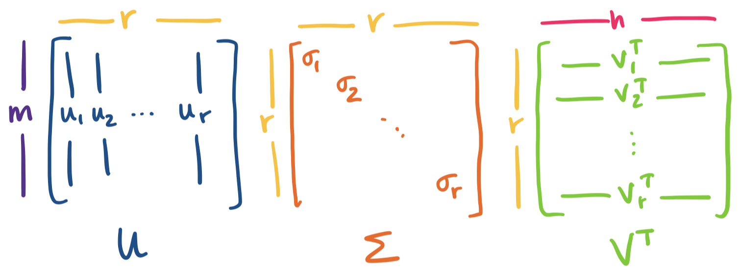
Let $A$ be an $m \times n$ matrix of rank $r$. Then \[A = U \Sigma V^T = \sigma_1 \mathbf u_1 \mathbf v_1^T + \cdots + \sigma_r \mathbf u_r \mathbf v_r^T,\] where $U$ is an orthogonal $m \times r$ matrix, $\Sigma$ is an $r \times r$ diagonal matrix, and $V$ is an orthogonal $n \times r$ matrix.
This factorization of $A$ is called the singular value decomposition of $A$. It's very important to emphasize: the SVD exists for any matrix, no matter its size, shape, invertibility, or anything else.
Let's dissect this.
Visually, we have the following picture:
We get something interesting immediately from this picture. Recall our view of matrix products. Whenever we have $A = BC$, we think of this both as $C$ describing how to combine columns of $B$ to construct columns of $A$ and $B$ describing how to combine rows of $C$ to construct rows of $A$.
We can apply this same interpretation to all matrix decompositions we've seen so far: $A = CR$, $A = LU$, $A = QR$, $A = X \Lambda X^{-1}$. We will apply this view to $A = U \Sigma V^T$ as well.
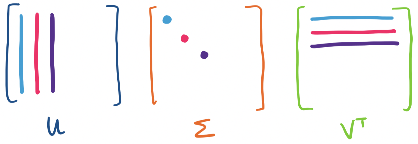
The last few we've seen are a bit puzzling because there are three matrices involved, but we can group them up into two matrices:
However, if we consider the other properties of $U$ and $V$, we can say something ever stronger.
We see that this decomposition is already paying off. Now, we make one further observation: the statement above casts $A$ as a sum of rank 1 matrices defined by the singular vectors of $A$. In particular, each singular value is associated with a specific left and right singular vector. It is this property that we will make use of in order to achieve our main goal: constructing low-rank approximations of $A$.
First, we note an analogy with eigenvalues. If $\mathbf x$ is an eigenvector, then we have $A \mathbf x = \lambda \mathbf x$. The singular values of a matrix give a similar relationship, though it connects two singular vectors, one on the left and one on the right, together rather than a single eigenvector: \[A \mathbf v = \sigma \mathbf u.\]
Let's see that this actually works out.
Consider the matrix $A = \begin{bmatrix} 1 & 2 & 0 \\ 0 & 1 & 2 \end{bmatrix}$. We have two singular vectors $\mathbf v_1 = \begin{bmatrix} 1 \\ 3 \\ 2 \end{bmatrix}$ and $\mathbf v_2 = \begin{bmatrix} -1 \\ -1 \\ 2 \end{bmatrix}$. This gives us \begin{align*} A\mathbf v_1 = \begin{bmatrix} 1& 2 & 0 \\ 0 & 1 & 2 \end{bmatrix} \begin{bmatrix} 1 \\ 3 \\ 2 \end{bmatrix} = \begin{bmatrix} 7 \\ 7 \end{bmatrix} \\ A\mathbf v_2 = \begin{bmatrix} 1& 2 & 0 \\ 0 & 1 & 2 \end{bmatrix} \begin{bmatrix} -1 \\ -1 \\ 2 \end{bmatrix} = \begin{bmatrix} -3 \\ 3 \end{bmatrix} \end{align*} We observe that $\mathbf v_1$ and $\mathbf v_2$ are orthogonal, but not orthonormal. The same holds for the resultant $A \mathbf v_1$ and $A \mathbf v_2$. We can easily normalize them: we see that $\|\mathbf v_1\| = \sqrt{14}$ and $\|\mathbf v_2\| = \sqrt{6}$. Normalizing $\mathbf v_1$ and $\mathbf v_2$ would lead us $\mathbf u_1 = \frac 1 {\sqrt 2} \begin{bmatrix} 1 \\ 1 \end{bmatrix}$ and $\mathbf u_2 = \frac 1{\sqrt 2} \begin{bmatrix} -1 \\ 1 \end{bmatrix}$, with singular values $\sigma_1 = \sqrt 7$ and $\sigma_2 = \sqrt 3$.
Putting this together, we have \[AV = \begin{bmatrix} 1& 2 & 0 \\ 0 & 1 & 2 \end{bmatrix} \begin{bmatrix} \frac 1 {\sqrt{14}} & -\frac 1 {\sqrt 6} \\ \frac 3 {\sqrt{14}} & -\frac 1 {\sqrt 6} \\ \frac 2 {\sqrt{14}} & \frac 2 {\sqrt 6} \end{bmatrix} = \frac 1 {\sqrt 2} \begin{bmatrix} 1 & -1 \\ 1 & 1 \end{bmatrix} \begin{bmatrix} \sqrt 7 & 0 \\ 0 & \sqrt 3 \end{bmatrix} = U \Sigma \] Since $V$ is orthonormal, we can write $A = U \Sigma V^T$ to get \[A = \begin{bmatrix} 1& 2 & 0 \\ 0 & 1 & 2 \end{bmatrix} = \frac 1 {\sqrt 2} \begin{bmatrix} 1 & -1 \\ 1 & 1 \end{bmatrix} \begin{bmatrix} \sqrt 7 & 0 \\ 0 & \sqrt 3 \end{bmatrix} \begin{bmatrix} \frac 1 {\sqrt{14}} & \frac 3 {\sqrt{14}} &\frac 2 {\sqrt{14}} \\ -\frac 1 {\sqrt 6} & -\frac 1 {\sqrt 6} & \frac 2 {\sqrt 6} \end{bmatrix}. \] When written in this way, we can see that we have \[A = \sqrt 7 \begin{bmatrix} \frac 1 {\sqrt 2} \\ \frac 1 {\sqrt 2} \end{bmatrix} \begin{bmatrix} \frac 1 {\sqrt{14}} & \frac 3 {\sqrt{14}} &\frac 2 {\sqrt{14}} \end{bmatrix} + \sqrt 3 \begin{bmatrix} -\frac 1 {\sqrt 2} \\ \frac 1 {\sqrt 2} \end{bmatrix} \begin{bmatrix}-\frac 1 {\sqrt 6} & -\frac 1 {\sqrt 6} & \frac 2 {\sqrt 6} \end{bmatrix}. \] or $A = \sigma_1 \mathbf u_1 \mathbf v_1^T + \sigma_2 \mathbf u_2 \mathbf v_2^T$.
In our example, we were given $\mathbf v_1$ and $\mathbf v_2$, but where do they come from in the first place? We want to achieve something like diagonalization, so as with diagonalization, we need to find our input and output vectors. For square matrices, we didn't have to think too hard about this: we could just take the eigenvectors and their inverses. For arbitrary matrices, we have a problem: one set of vectors belongs to $\mathbb R^m$ and the other belongs to $\mathbb R^n$. However, we will use our standard trick when it comes to rectangular matrices: multiply them by their transpose.
In our case, we will require both $A^TA$ and $AA^T$. If $A$ is $m \times n$, then we observe that $A^TA$ is an $n \times n$ matrix and $AA^T$ is an $m \times m$ matrix. Another special thing about these matrices is that they are symmetric. Recall that a symmetric matrix is one that is the same if we transpose it—that is, $A = A^T$.
Why is this important? Recall that we require that an $n \times n$ matrix has $n$ independent eigenvectors, so it's not the case that we can always diagonalize a matrix. This situation is a bit like the LU factorization, where only invertible matrices have LU decompositions. But symmetric matrices give us a fairly strong decomposition result, called the Spectral Theorem.
Let $S$ be a real symmetric matrix. Then $S = Q\Lambda Q^T$ for some orthogonal matrix $Q$.
Suppose $S$ has a nonzero eigenvalue and a zero eigenvalue. Then $S \mathbf x = \lambda \mathbf x$ and $S \mathbf y = 0 \mathbf y$. These tell us that
This doesn't seem to help us because the column space and null space are not orthogonal complements. However, $S$ is symmetric—this means its row space is the same as its column space. This is enough to give us that $\mathbf x$ and $\mathbf y$ are orthogonal.
But what if we have another non-zero eigenvalue $\alpha$? We have $S \mathbf y = \alpha \mathbf y$. So consider $S - \alpha I$. This gives us $(S - \alpha I) \mathbf y = \mathbf 0$ and $(S - \alpha I) \mathbf x = (\lambda - \alpha)\mathbf x$. Then $\mathbf y$ is in the null space of $S - \alpha I$ and $\mathbf x$ is in the column space of $S - \alpha I$, which is the row space of $S - \alpha I$. So the two vectors are orthogonal.
There are a few things to note here.
Consider the matrix $A = \begin{bmatrix} 2 & -1 & -1 \\ -1 & 2 & -1 \\ -1 & -1 & 2 \end{bmatrix}$. Its characteristic polynomial is $-\lambda(\lambda-3)^2$, so we have $\lambda = 0, 3$.
For $\lambda = 0$, we have $\begin{bmatrix} 2 & -1 & -1 \\ -1 & 2 & -1 \\ -1 & -1 & 2 \end{bmatrix} \mathbf x = 0$. This has rref $\begin{bmatrix} 1 & 0 & -1 \\ 0 & 1 & -1 \\ 0 & 0 & 0 \end{bmatrix}$, which gives us a special solution of $\begin{bmatrix} 1 \\ 1 \\ 1 \end{bmatrix}$.
For $\lambda = 3$, we have $\begin{bmatrix} -1 & -1 & -1 \\ -1 & -1 & -1 \\ -1 & -1 & -1 \end{bmatrix} \mathbf x = 0$. This matrix has an rref of $\begin{bmatrix} 1 & 1 & 1 \\ 0 & 0 & 0 \\ 0 & 0 & 0 \end{bmatrix}$, which gives us special solutions of $\begin{bmatrix} -1 \\ 1 \\ 0 \end{bmatrix}, \begin{bmatrix} -1 \\ 0 \\ 1 \end{bmatrix}$.
If we put these together, we have $\Lambda = \begin{bmatrix} 3 & 0 & 0 \\ 0 & 3 & 0 \\ 0 & 0 & 0 \end{bmatrix}$ and $X = \begin{bmatrix} -1 & -1 & 1 \\ 1 & 0 & 1 \\ 0 & 1 & 1 \end{bmatrix}$. However, we now need to take the extra step of ensuring our eigenvectors are orthonormal. As alluded to in the proof, we don't need to worry about orthogonalizing against all of the vectors, since those with different eigenvalues are already guaranteed to be orthogonal—any such vectors only need to be normalized.
The trickiness comes in when we have multiple eigenvectors for one eigenvalue. We notice that the special solutions we get from solving for the null space are not generally orthogonal. Luckily, this amounts to finding an orthonormal basis for the null space, which we can easily do by applying Gram–Schmidt.
So we take $\begin{bmatrix} -1 \\ 0 \\ 1 \end{bmatrix}$ and use it to find a vector orthogonal to $\begin{bmatrix}-1 \\ 1 \\ 0 \end{bmatrix}$. We get \[\begin{bmatrix} -1 \\ 0 \\ 1 \end{bmatrix} - \begin{bmatrix} -1 \\ 1 \\ 0 \end{bmatrix} \frac{\begin{bmatrix} -1 & 1 & 0 \end{bmatrix} \begin{bmatrix} -1 \\ 0 \\ 1 \end{bmatrix}}{\begin{bmatrix} -1 & 1 & 0 \end{bmatrix} \begin{bmatrix} -1 \\ 1 \\ 0 \end{bmatrix}} = \begin{bmatrix} -1 \\ 0 \\ 1 \end{bmatrix} - \begin{bmatrix} -1 \\ 1 \\ 0 \end{bmatrix} \frac 1 2 = \begin{bmatrix} -\frac 1 2 \\ -\frac 1 2 \\ 1 \end{bmatrix}. \]
So now that our eigenvectors are orthogonalized, we normalize them to get \[Q = \begin{bmatrix} -\frac 1 {\sqrt 2} & -\frac 1 {\sqrt 6} & \frac 1 {\sqrt 3} \\ \frac 1 {\sqrt 2} & -\frac 1 {\sqrt 6} & \frac 1 {\sqrt 3} \\ 0 & \frac 2{\sqrt 6} & \frac 1 {\sqrt 3} \end{bmatrix}.\]