Eigenvectors present us with another opportunity to decompose a matrix. Suppose first that we happen to have an $n \times n$ matrix $A$ with $n$ independent eigenvectors (not obvious that we can always do this!). We use our usual trick for working with several vectors: make them the columns of a matrix. What do we gain from this?
First, remember that if we have an eigenvector $\mathbf x$, we have that $A \mathbf x = \lambda \mathbf x$. Now, suppose we take each eigenvector $\mathbf x_1, \dots, \mathbf x_n$ and put them in a matrix $X$. What is the matrix product $AX$? If we apply the usual column-centric view of matrix multiplication, we have \[AX= A \begin{bmatrix} \quad \\ \mathbf x_1 & \cdots & \mathbf x_n \\ \quad \end{bmatrix} = \begin{bmatrix} \quad \\ \lambda_1 \mathbf x_1 & \cdots & \lambda_n \mathbf x_n \\ \quad \end{bmatrix}.\] To see why this is the case, recall that the $i$th column of $X$ determines the $i$th column of the product $AX$ and it is equal to $A$ multiplied by that column. In this case, the $i$th column of $X$ is $\mathbf x_i$, so $A \mathbf x_i = \lambda_i \mathbf x_i$.
To get the decomposition we're looking for, we now decompose the right hand side. We have \[\begin{bmatrix} \quad \\ \lambda_1 \mathbf x_1 & \cdots & \lambda_n \mathbf x_n \\ \quad \end{bmatrix} = \begin{bmatrix} \quad \\ \mathbf x_1 & \cdots & \mathbf x_n \\ \quad \end{bmatrix} \begin{bmatrix} \lambda_1 & & \\ & \ddots & \\ & & \lambda_n \end{bmatrix} = X \Lambda.\] This is fairly straightforward: our product is simply the rhs of the eigenvector equation, so we split up the eigenvectors and eigenvalues. We denote the eigenvalue matrix by $\Lambda$, which is the uppercase version of $\lambda$. This gives us the following theorem.
Let $A$ be an $n \times n$ matrix with $n$ linearly independent eigenvectors. Then $AX = X \Lambda$, where $X$ is the matrix of eigenvectors of $A$ and $\Lambda$ is a diagonal matrix of eigenvalues of $A$.
One thing to note here is that $X$ is gives us a basis for the column space of $A$. If the eigenvectors have nonzero eigenvalues, they are in the column space of $A$ (since $A \mathbf x = \lambda \mathbf x)$. If we have $n$ such linearly independent vectors, this gives us a basis.
This gives us a way to satisfy the following definition:
A matrix $A$ is diagonalizable if there exists an invertible matrix $P$ and a diagonal matrix $D$ such that $A = PDP^{-1}$.
So we have that $P = X$, the matrix of eigenvectors, and $D = \Lambda$, the matrix of eigenvalues.
Why is this useful? Remember that a requirement is that $A$ has $n$ linearly independent eigenvectors. This means that the columns of $X$ are all independent—that is, $X$ is invertible. We have the following corollary:
Let $A$ be an $n \times n$ matrix with $n$ linearly independent eigenvectors. Then $A = X \Lambda X^{-1}$ and $\Lambda = X^{-1} A X$.
Consider the matrix $A = \begin{bmatrix} -1 & 0 & -8 \\ 0 & -1 & 8 \\ 0 & 0 & 3 \end{bmatrix}$. Since $A$ is upper triangular, we have that the eigenvalues of $A$ are $-1$ (with multiplicity 2) and $3$.
First, we solve for $\lambda = 3$. In this case, we have the equation \[\begin{bmatrix} -4 & 0 & -8 \\ 0 & -4 & 8 \\ 0 & 0 & 0 \end{bmatrix} \mathbf x = \mathbf 0.\] The rref of this matrix is $\begin{bmatrix} 1 & 0 & 2 \\ 0 & 1 & -2 \\ 0 & 0 & 0 \end{bmatrix}$, so the special solution gives us $\begin{bmatrix} -2 \\ 2 \\ 1 \end{bmatrix}$, which is our eigenvector for $\lambda = 3$.
Next, we consider $\lambda = -1$. We have the equation \[\begin{bmatrix} 0 & 0 & -8 \\ 0 & 0 & 8 \\ 0 & 0 & 4 \end{bmatrix} \mathbf x = \mathbf 0.\] The rref of this matrix is $\begin{bmatrix} 0 & 0 & 1 \\ 0 & 0 & 0 \\ 0 & 0 & 0 \end{bmatrix}$. This gives us a special solution of $\begin{bmatrix} 1 \\ 0 \\ 0 \end{bmatrix}, \begin{bmatrix} 0 \\ 1 \\ 0 \end{bmatrix}$.
This is good because we now have three linearly independent eigenvectors. We can now construct $X = \begin{bmatrix} 1 & 0 & -2 \\ 0 & 1 & 2 \\ 0 & 0 & 1 \end{bmatrix}$, which goes together with $\Lambda = \begin{bmatrix} -1 & 0 & 0 \\ 0 & -1 & 0 \\ 0 & 0 & 3 \end{bmatrix}$.
First, a pressing question: what order do these go in? Based on our "proof" from above, it actually doesn't matter: we can choose an arbitrary order for $X$ and the result of $AX$ should be $X \Lambda$. So all we need to do is make sure that the correct eigenvalues are paired with the right eigenvectors and stick with that order.
To complete the factorization, we compute $X^{-1} = \begin{bmatrix} 1 & 0 & 2 \\ 0 & 1 & -2 \\ 0 & 0 & 1 \end{bmatrix}$.
In summary, we have \[A = \begin{bmatrix} -1 & 0 & -8 \\ 0 & -1 & 8 \\ 0 & 0 & 3 \end{bmatrix} = \begin{bmatrix} 1 & 0 & -2 \\ 0 & 1 & 2 \\ 0 & 0 & 1 \end{bmatrix} \begin{bmatrix} -1 & 0 & 0 \\ 0 & -1 & 0 \\ 0 & 0 & 3 \end{bmatrix} \begin{bmatrix} 1 & 0 & 2 \\ 0 & 1 & -2 \\ 0 & 0 & 1 \end{bmatrix}.\]
This example shows us that although unique eigenvalues guarantee that we have linearly independent eigenvectors, they are not necessary. Because of this, there are actually two different notions of multiplicity:
These can be different: it may be the case that the geometric multiplicity is less than the algebraic multiplicity. In this case, we do not have enough linearly independent eigenvectors to diagonalize our matrix. However, the geometric multiplicity can only be at most the algebraic multiplicity and no greater.
Consider the matrix $A = \begin{bmatrix} -1 & 4 & -8 \\ 0 & -1 & 4 \\ 0 & 0 & 3 \end{bmatrix}$. This matrix has the same eigenvalues as our example from before. This time we will note that the eigenvalue $\lambda = -1$ has algebraic multiplicity 2, since it appears twice as a root of the characteristic polynomial. We will solve for the eigenvectors for $\lambda = -1$.
We arrive at a matrix $\begin{bmatrix} 0 & 4 & -8 \\ 0 & 0 & 4 \\ 0 & 0 & 4 \end{bmatrix}$. The rref for this matrix is $\begin{bmatrix} 0 & 1 & 0 \\ 0 & 0 & 1 \\ 0 & 0 & 0 \end{bmatrix}$. Notice that there are two pivot columns. This means that the null space of this matrix has only one dimension, and so there is only one eigenvector, $\begin{bmatrix} 1 \\ 0 \\ 0 \end{bmatrix}$. Therefore, the geometric multiplicity of $\lambda = -1$ is 1.
This is important because it tells us that not every matrix is diagonalizable. Now that we've been at this course for a while, you might wonder what is wrong with these matrices, but in fact, there's nothing obvious—for example, notice that our matrix is a perfectly fine upper triangular matrix with linearly independent columns. No, diagonalization just happens to be a property that depends on eigenvectors, which we haven't really worked with much until now.
Let's go back to the original motivation for this problem and see how it's resolved. We have the following result that follows right from our decomposition.
Let $A$ be an $n \times n$ matrix that has diagonalization $A = X \Lambda X^{-1}$. Then $A^k = X \Lambda^k X^{-1}$.
To see this, we expand $A^k$ into $(X \Lambda X^{-1})(X \Lambda X^{-1}) \cdots (X \Lambda X^{-1})$. Notice that in between each factor, we have $X^{-1} X = I$.
One example of data that may appear in the form of a square matrix are graphs. Graphs are a common mathematical structure in discrete mathematics and computer science for representing structures like networks.
A graph $G = (V,E)$ is a set of vertices $V$ and edges $E$, which are pairs $(u,v)$ that join vertices $u$ and $v$. Graphs may be directed or undirected.
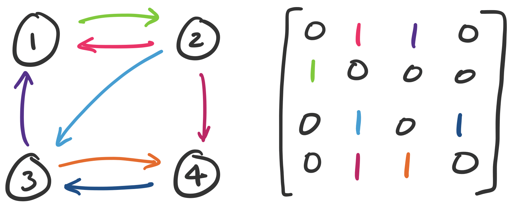
We can represent graphs as matrices by defining an adjacency matrix. Suppose each vertex is labelled $1$ through $n$. Then entry $a_{ij}$ is set to 1 if there is an edge $(i,j)$ in our graph and 0 otherwise.
Consider the following graph and let $A$ be its adjacency matrix. The entries of the matrix are colour-coded with the corresponding edges.
The matrix representation of a graph can be quite handy. For example, we can determine reachability by using matrix multiplication.
The number of paths from vertex $u$ to vertex $v$ of length exactly $k$ is $A_{uv}^k$.
To see this, consider the following matrices for our graph above. \[ A^2 = \begin{bmatrix} 1 & 1 & 0 & 1 \\ 0 & 1 & 1 & 0 \\ 1 & 1 & 1 & 0 \\ 1 & 1 & 0 & 1 \end{bmatrix} \quad A^3 = \begin{bmatrix} 1 & 2 & 2 & 0 \\ 1 & 1 & 0 & 1 \\ 1 & 2 & 1 & 1 \\ 1 & 2 & 2 & 0 \end{bmatrix} \quad A^4 = \begin{bmatrix} 2 & 3 & 1 & 2 \\ 1 & 2 & 2 & 0 \\ 2 & 3 & 2 & 1 \\ 2 & 3 & 1 & 2 \end{bmatrix}. \]
A result from graph theory says that in a graph of $n$ vertices, if a vertex $v$ is reachable from vertex $u$, then there is always a path of length at most $n$. This means that we can test connectivity by considering $A^n$. Realistically, this is quite expensive, even if we diagonalize the matrix: for a graph of $n$ vertices, our adjacency matrix is $n \times n$. If we diagonalize our matrix, we still perform at least one matrix multiplication which is at worst something like $O(n^3)$ operations. Simple graph search algorithms like breadth- and depth-first search run linearly in the number of edges and vertices.
Another way to use the matrix is instead of using a binary entry (1 or 0) to denote the presence of an edge, we can instead assign it a weight. This leads us to the following example.
A (column-)stochastic matrix, also called a Markov matrix is a matrix in which the entries of the matrices are probabilities (i.e. they are real numbers between 0 and 1) and the sum of the entries of each column is 1.
We can consider one of these matrices $A = \begin{bmatrix} \frac 1 2 & \frac 1 4 \\ \frac 1 2 & \frac 3 4 \end{bmatrix}$. This matrix represents the following Markov chain:
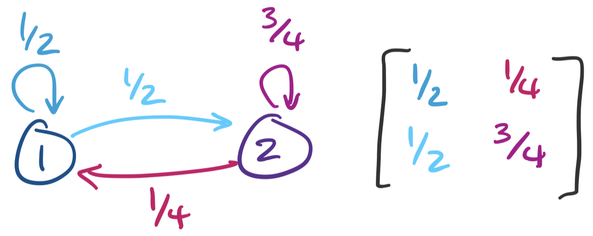
From this, we see that we can view a Markov chain as a graph with probability-weighted edges. We label each vertex of our graph 1 through $n$ and label entry $i,j$ by the weight of the edge from vertex $i$ to vertex $j$.
Traditionally, the question that we want an answer for is what this system looks like as time goes on. In other words, when we take, say, 100 or 1000 or 10000 steps on this Markov chain, where do we end up? To answer this, we have to ask what $A^{10000}$ is. This is an expensive computation to do directly (especially without the help of a computer), so we diagonalize $A$.
First, we see that the characteristic polynomial of $A$ is $\lambda^2 - \frac 5 4 \lambda + \frac 1 4$, which gives us roots $\lambda = 1, \frac 1 4$. This gives us \begin{align*} \lambda &= 1: & \begin{bmatrix} - \frac 1 2 & \frac 1 4 \\ \frac 1 2 & - \frac 1 4 \end{bmatrix} \mathbf x &= \mathbf 0 & \mathbf x &= \begin{bmatrix} \frac 1 2 \\ 1 \end{bmatrix} \\ \lambda & = \frac 1 4: & \begin{bmatrix} \frac 1 4 & \frac 1 4 \\ \frac 1 2 & \frac 1 2 \end{bmatrix} \mathbf x &= \mathbf 0 & \mathbf x &= \begin{bmatrix} -1 \\ 1 \end{bmatrix} \end{align*}
This gives us $X = \begin{bmatrix} 1 & -1 \\ 2 & 1 \end{bmatrix}$ and $\Lambda = \begin{bmatrix} 1 & 0 \\ 0 & \frac 1 4 \end{bmatrix}$. We have that $X^{-1} = \begin{bmatrix} \frac 1 3 & \frac 1 3 \\ - \frac 2 3 & \frac 1 3 \end{bmatrix}$. This gives us \[A^k = \begin{bmatrix} 1 & -1 \\ 2 & 1 \end{bmatrix} \begin{bmatrix} 1 & 0 \\ 0 & \frac 1 4 \end{bmatrix}^k \begin{bmatrix} \frac 1 3 & \frac 1 3 \\ -\frac 2 3 &\frac 1 3 \end{bmatrix}.\]
Again, the question we want to know is what happens when we take many steps. In other words, what happens when $k$ gets very, very large? We take a page from calculus and think about what happens when $k \to \infty$. The effect of $k$ on our diagonal matrix is this: \[A^k = \begin{bmatrix} 1 & -1 \\ 2 & 1 \end{bmatrix} \begin{bmatrix} 1^k & 0 \\ 0 & \left(\frac 1 4\right)^k \end{bmatrix} \begin{bmatrix} \frac 1 3 & \frac 1 3 \\ -\frac 2 3 &\frac 1 3 \end{bmatrix}.\] We recall that $1^k = 1$ no matter how large $k$ gets. However, $\frac 1 {4^k}$ shrinks more and more as $k$ gets larger. As a result, we can treat it as though it becomes 0. So as $k \to \infty$, our system looks more like \[A^k = \begin{bmatrix} 1 & -1 \\ 2 & 1 \end{bmatrix} \begin{bmatrix} 1 & 0 \\ 0 & 0 \end{bmatrix} \begin{bmatrix} \frac 1 3 & \frac 1 3 \\ -\frac 2 3 &\frac 1 3 \end{bmatrix} = \begin{bmatrix} \frac 1 3 & \frac 1 3 \\ \frac 2 3 & \frac 2 3 \end{bmatrix}.\]
This result tells us that as we take more steps in the Markov chain, we have a higher chance of ending up in state 2. This makes sense: while there's an equal probability of going to either state when in state 1, we have a higher chance of staying in state 2 once we've entered it.
Here, we see that diagonalization provides us with information about the behaviour of this system even without computing the matrix.