Let's think a bit about geometry, which is really about putting mathematical objects in some kind of space. Most people are first introduced to vectors in this way, usually in a physics class. Typically, we think of vectors geometrically in 2 and 3 dimensions over real scalars because that is the world that we inhabit. Doing this can be helpful for developing intiution for how vectors behave beyond two or three dimensions or things other than real numbers—you'll see a lot of people framing concepts geometrically even in higher dimensions. A lot of things in mathematics and computer science become very difficult once you go beyond three dimensions, but linear algebra happens not be one of them—a lot of ideas happen to generalize very nicely.
One obvious property of a vector when we draw it out is the idea of the length of a vector. This corresponds with the "magnitude" part of a vector in the physics conception (the other part being the "direction").
The length of a vector $\mathbf v = \begin{bmatrix} v_1 \\ v_2 \\ \vdots \\ v_n\end{bmatrix}$ is \[\|\mathbf v\| = \sqrt{v_1^2 + v_2^2 + \cdots + v_n^2}.\]
The idea of length is evocative of geometry—it's the "length" of the arrow that represents the vector. This is just the usual Euclidean notion of length, which is just how "far" away it is from the origin. One fun thing to do is to think about what other kinds of "length" we might be able to define on vectors and still have such a notion still make some kind of sense—the proper mathematical terminology for such functions is a norm. Here, our definition of the length of the vector is also called the Euclidean norm.
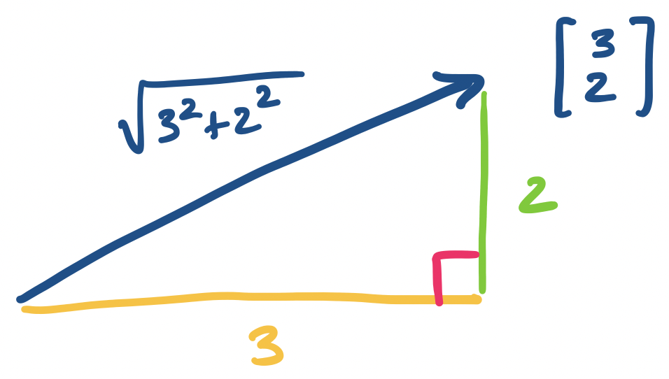
Consider the vector $\mathbf v = \begin{bmatrix} 3 \\ 2 \end{bmatrix}$. By definition, its length is $\sqrt{3^2 + 2^2} = \sqrt{13}$.
The reason why this makes sense as a definition for length is pretty clear in two dimensions if you remember how triangles work and it turns out this idea carries over to higher dimensions.
The concept of the length of a vector is important because we can have multiple vectors in the same "direction" but of different lengths. In a sense, these are all the same "kind" of vector, since they can be expressed as a very simple linear combination of each other—via scalar multiplication (hence, "scalar"). This leads to the concept of a unit vector, which can be thought of as a "standard" vector for all of these vectors headed in the same direction.
A unit vector $\mathbf v$ is a vector with length $1$.
We can take any vector and find a unit vector in the same direction by "normalizing" it.
Let $\mathbf v$ be a vector. Then $\frac 1 {\|\mathbf v\|} \mathbf v$ is a unit vector in the same direction as $\mathbf v$.
Notice here that $\frac{1}{\|\mathbf v \|}$ is a scalar: the length of $\mathbf v$ is a real number and its inverse is a real number, so we're really scaling the vector. Once we know this, it becomes a bit more clear what's happening intuitively. We want a vector that's going in the same direction as $\mathbf v$, so let's scale it down by its length—this should result in a vector that has length 1.
Once we have the notion of length, we can also think about distances between vectors.
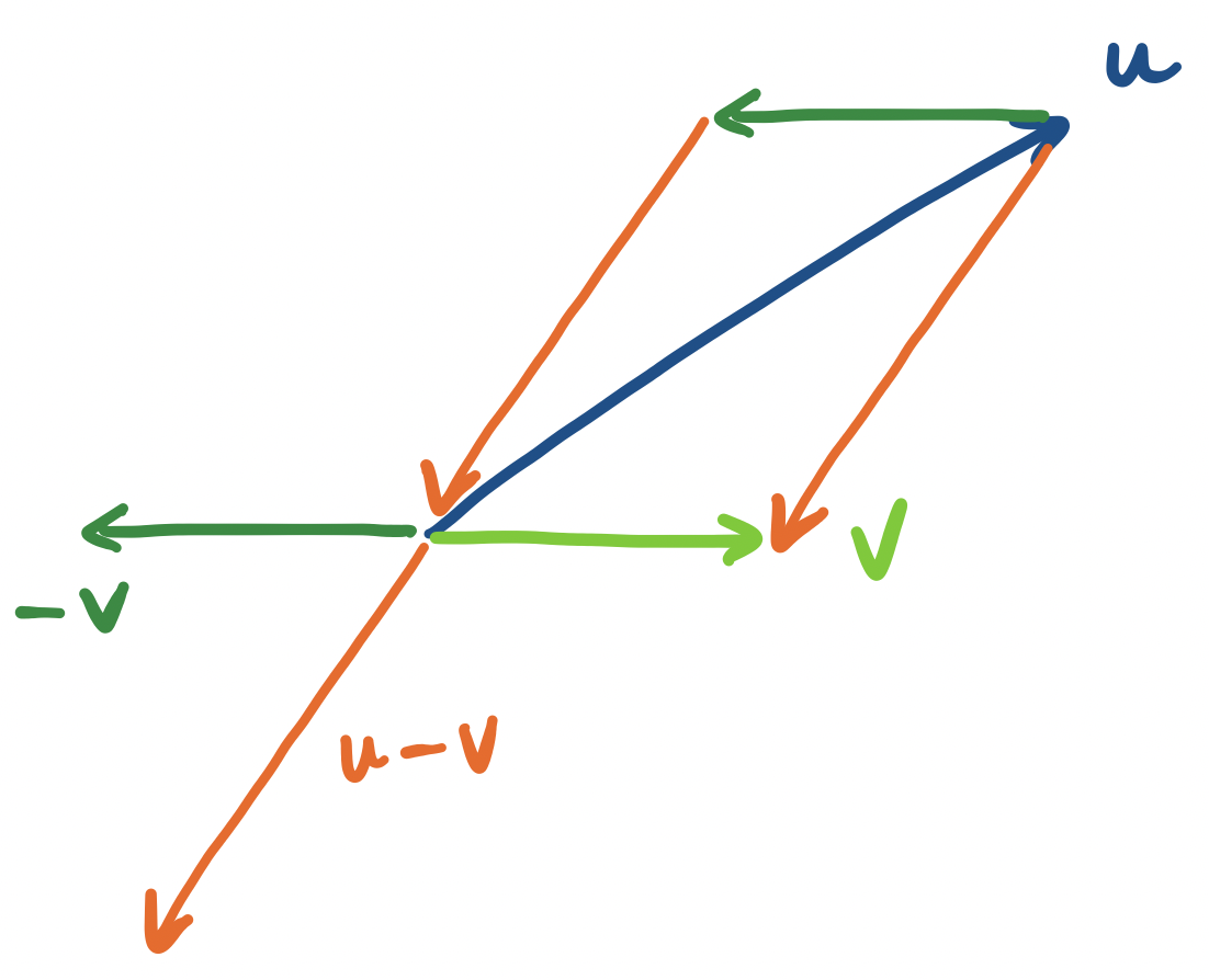
Let $\mathbf u$ and $\mathbf v$ be vectors. The distance between $\mathbf u$ and $\mathbf v$ is $\|\mathbf u - \mathbf v \|$.
It's worth thinking about what this definition is saying. First, we notice that $\mathbf u - \mathbf v$ is a vector: subtraction is just a combination of addition and scaling one vector by $-1$. So we define the distance to be the length of the vector that takes us from $\mathbf u$ to $\mathbf v$.
Distances are useful because in many applications, we can treat the distance as a similarity measure. Suppose a vector $\mathbf v = \begin{bmatrix} 2.3 \\ 4.22 \\ -1.7 \end{bmatrix}$ represents, say, a Spotify user and the numbers are some computed score for how much they like a particular artist or genre. If we associate each user with a vector, we can ask questions like how similar one user is to another user. One way to do this with the definitions we have so far is to compute the distance between the two vectors.
This notion of similarity is pretty straightforward and is often used in many applications. It makes sense because it's an obvious definition, but it's also easy to visualize: of course two things are more similar if they're closer together.
Now, we introduce a very useful quantity: the dot product of two vectors. This is what you would get if you were to say wait a minute—we don't really have multiplication of vectors, because scalar multiplication is just multipliying a number with a vector.
The dot product of vectors $\mathbf u = \begin{bmatrix}u_1 \\ u_2 \\ \vdots \\ u_n \end{bmatrix}$ and $\mathbf v = \begin{bmatrix} v_1 \\ v_2 \\ \vdots \\ v_n \end{bmatrix}$ is \[\mathbf u \cdot \mathbf v = u_1 v_1 + u_2 v_2 + \cdots + u_n v_n.\]
It's important here that the vectors have the same dimension (i.e. they have the same number of entries). We want the vectors to "live" in the same "space", which means, for our purposes, that they have the same number of dimensions. This notion will be formalized later on.
Let $\mathbf u = \begin{bmatrix}4 \\ 2 \\ -1\end{bmatrix}$ and $\mathbf v = \begin{bmatrix} 2 \\ -3 \\ 5 \end{bmatrix}$. Then \[\mathbf u \cdot \mathbf v = 4 \times 2 + 2 \times -3 + -1 \times 5 = -3.\]
Notice that the dot product is a scalar.
What can the dot product tell us? Suppose again that our vectors represent, say, a Spotify user's tastes in various genres of music. We've already seen that we can compare two users' tastes by considering the distance between their "taste vectors". But here's something we can do with the dot product.
Suppose that we would like to identify certain users with certain mixes of tastes. Let's say that a vector $\begin{bmatrix} v_1 \\ v_2 \\ v_3 \end{bmatrix}$ represents a user's preference or not for rock, ska, and Eurobeat, respectively. We can design a "template" user that prefers rock, detests ska, and is indifferent to Eurobeat by the vector $\begin{bmatrix} 100 \\ -100 \\ 0 \end{bmatrix}$. Then taking the dot product of a vector with this template, $100v_1 - 100v_2 + 0v_3$, will give us a scalar quantity. The larger that quantity is, the more similar the user is to our template, and the smaller (i.e. negative) it is, the less similar they are. In some sense, our template "weights" the genre scores.
From this it seems like the numbers make sense, but we can also jump back to geometry to round out our understanding of why this works.
One interesting observation is that the length of a vector is related to the dot product: \[\|\mathbf v\|^2 = \mathbf v \cdot \mathbf v.\] Notice that this means that a unit vector $\mathbf v$ has $\mathbf v \cdot \mathbf v = 1$.
This leads to the question of what happens when $\mathbf u \cdot \mathbf v = 0$. Of course, if $\mathbf v \cdot \mathbf v = 0$, this means that we must have $\mathbf v = 0$. But otherwise, we get the following.
For any two nonzero vectors $\mathbf u$ and $\mathbf v$, $\mathbf u \cdot \mathbf v$ if and only if $\mathbf u$ is perpendicular to $\mathbf v$.
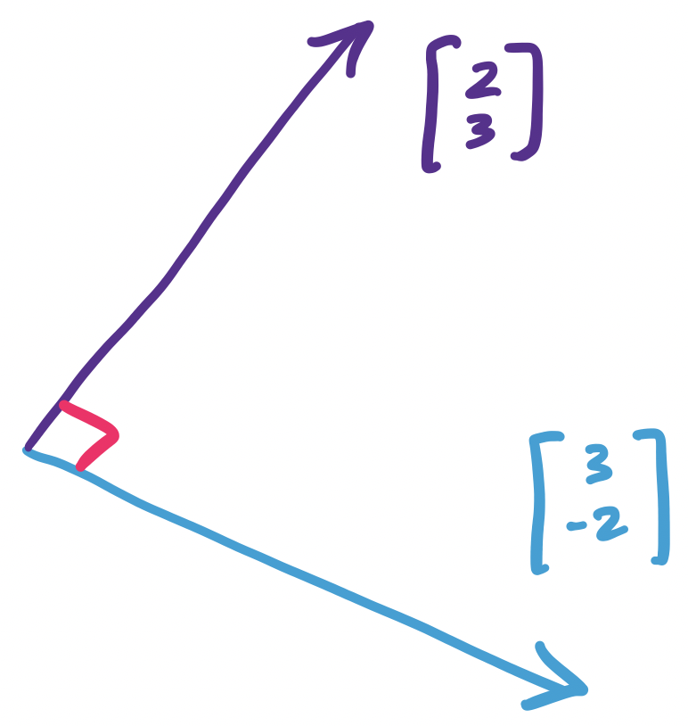
Let $\mathbf u = \begin{bmatrix} 3 \\ -2 \end{bmatrix}$. We claim that $\mathbf v = \begin{bmatrix} 2 \\ 3 \end{bmatrix}$ is perpendicular to $\mathbf u$. We can verify by this by checking their dot product:
\[\mathbf u \cdot \mathbf v = 3 \times 2 + (-2) \times 3 = 0.\]
Indeed, if we draw this out, we get:
Why does this work? When we view vectors geometrically, we can consider the "angle" that is formed between them. The dot product happens to be proportional to the cosine of this angle.
For all vectors $\mathbf u$ and $\mathbf v$, $\mathbf u \cdot \mathbf v = \|\mathbf u\| \|\mathbf v\| \cos \theta$.
We won't prove this, but this gives us an idea for why the dot product can capture a notion of similarity—but based on the direction of the vectors rather than their distance.
Recall that the cosine function takes as input some angle and produces some real number in the interval $[-1,1]$. The important points to keep in mind are:
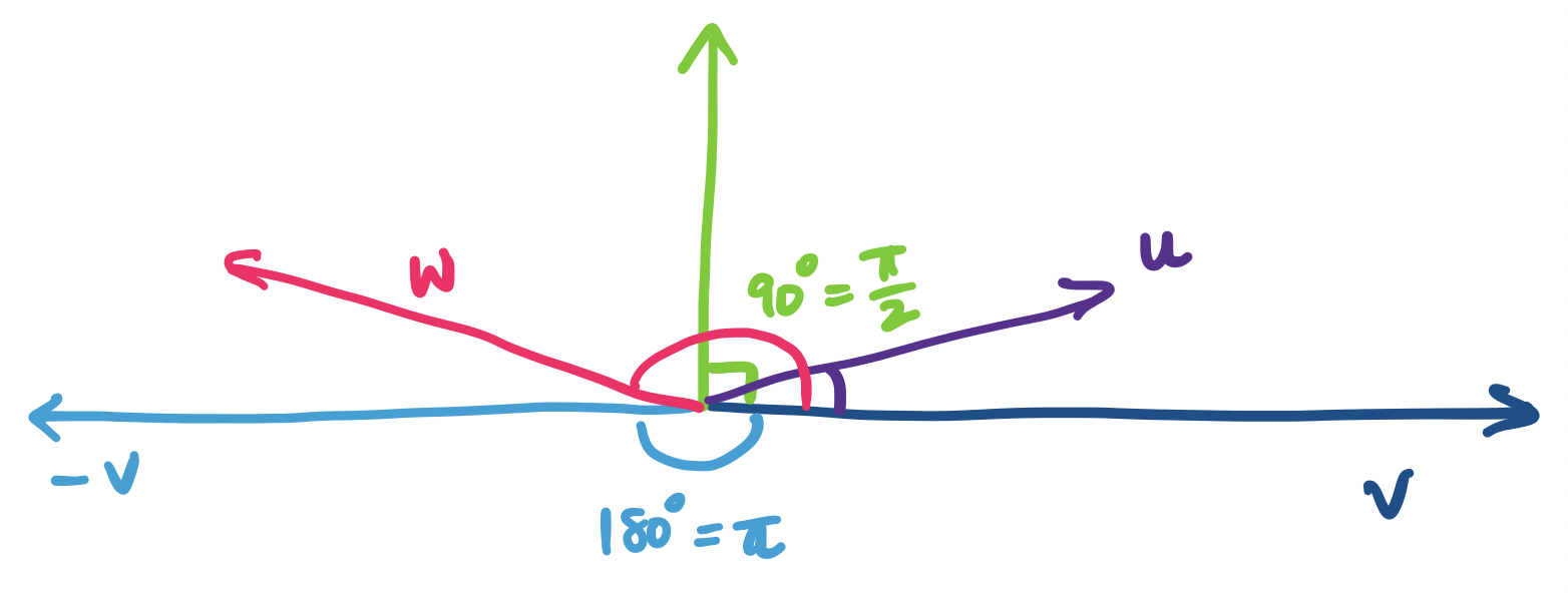
That is, the dot product can capture how similar two vectors are in terms of their direction. If the two vectors are pointing in roughly the same direction, their dot product will be positive; otherwise if they're pointing away from each other, it'll be negative. Notice that the closer they are to either the original direction or its opposite, the "intensity" of $\cos \theta$ increases. If the vectors are completely orthogonal, then we get 0.
In the above diagram, $\mathbf u \cdot \mathbf v$ is positive, since its angle is between 0 and 90 degrees, while $\mathbf v \cdot \mathbf w$ is negative, since its angle is between 90 and 180 degrees. If $\mathbf u$ is closer to $\mathbf v$, the cosine of the angle is closer to 1 and if it is closer to the green vector, the cosine of the angle gets closer to 0. Similarly, if $\mathbf w$ is closer to $\mathbf -v$, the cosine of the angle it makes with $\mathbf v$ gets closer to $-1$, while the closer it is to the green vector, the closer the cosine of its angle gets to 0, but on the negative side.
This makes sense for a two-dimensional vector but this property still holds in higher dimensions. The reason for this is pretty simple: if I have two vectors in any number of dimensions, I can always find a plane that they lie on and figure out an angle between them.
It's maybe a bit early for this and we don't really get into it much, but it's interesting to note that these are not arbitrary definitions. Instead, they are consequences of the idea that vectors are things that we can add and scale. If we used weirder scalars, we would be able to come up with similarly appropriate definitions. (These more general dot products have a name—they're called inner products and the dot product is a specific instance of an inner product)
Linear algebra is built around the two operations vector addition and scalar multiplication. It's all you need! This tells us something very neat: that the only thing we need to know how to do is add two things together and scale them. Just from these two operations, we get an enormous amount of utility.
Again, we note that the ability to add and scale vectors is what separates them from tuples. Indeed, a formal definition of a vector is an object that allows us to apply these two operations. This means that it's not the case that vectors are just arbitrary ordered collections of items—these items need to be able to be added and scaled.
How do we begin using these? Well, these two operations already give us something very neat: we can create all kinds of vectors by using other vectors and applying these operations to them.
Let $\mathbf u = \begin{bmatrix}1 \\ 3 \end{bmatrix}$ and $\mathbf v = \begin{bmatrix} -5 \\ 2 \end{bmatrix}$. Then $2\mathbf u - 3 \mathbf v = \begin{bmatrix} 17 \\ -3 \end{bmatrix}$.
This is an important idea, so we should call it something.
A vector $\mathbf v$ is a linear combination of vectors $\mathbf u_1, \dots, \mathbf u_n$ if there exist scalars $a_1, \dots, a_n$ such that \[\mathbf v = a_1 \mathbf u_1 + \cdots + a_n \mathbf u_n.\]
In other words, $\mathbf v$ can be expressed as the sum of some vectors and some scaling.
Here, we have an interesting question that crops up. Let's say that we have a bunch of vectors. What other vectors can we make with these? More formally, what is the set of vectors that are linear combinations of our original set of vectors?
These seem like arbitrary questions that are only interesting to mathematicians, and for a long time, you would've been right. However, computer science lets us find clever ways to make use of these questions.
For example, suppose we have a collection of objects. These objects have properties that can be expressed numerically. We can treat such an object as a vector of these properties. And if we have a bunch of these objects, we have a bunch of vectors. These objects have some similarities with each other.
Here, we introduce the other big object in the study of linear algebra: the matrix. We just saw the idea of thinking about collections of vectors. Matrices are a convenient object that puts these vectors together so we can consider them as one "thing".
An $m \times n$ matrix is a rectangle of $m \times n$ scalars. Such a matrix has $m$ rows and $n$ columns.
Here are some examples of matrices: \[\begin{bmatrix} 3 \end{bmatrix}, \begin{bmatrix} -7 \\ 6 \\ 5 \end{bmatrix}, \begin{bmatrix}3 & 1 & -5 \end{bmatrix}, \begin{bmatrix}2 & 4 \\ 3 & 4 \end{bmatrix}, \begin{bmatrix}3 & 4 & 6 \\ 9 & 6 & 1 \end{bmatrix}.\]
We refer to a particular entry of the matrix by two indices $i$ and $j$, where $i$ is the row and $j$ is the column. So if $A = \begin{bmatrix}2 & 3 \\ 4 & -1 \\ 5 & 1 \end{bmatrix}$, then $A_{3,1} = 5$ and $A_{1,2} = 3$.
Like vectors, the "real" formal definition of a matrix is much more general and less recognizable than what most people would consider to be a matrix. And like the formal definition of vectors, the formal definition of a matrix is not so important in our context.
First, we'll consider what we can do with a matrix. In other words, what are the operations we want to perform on it? One thing we can do is multiply a matrix by a vector to get another vector.
Let $A = \begin{bmatrix} 2 & -4 \\ -3 & 4 \end{bmatrix}$ and $\mathbf v = \begin{bmatrix} 1 \\ 5 \end{bmatrix}$. We want to compute the product \[A \mathbf v = \begin{bmatrix} 2 & -4 \\ -3 & 4 \end{bmatrix}\begin{bmatrix} 1 \\ 5 \end{bmatrix} = \begin{bmatrix} -18 \\ 17 \end{bmatrix}.\]
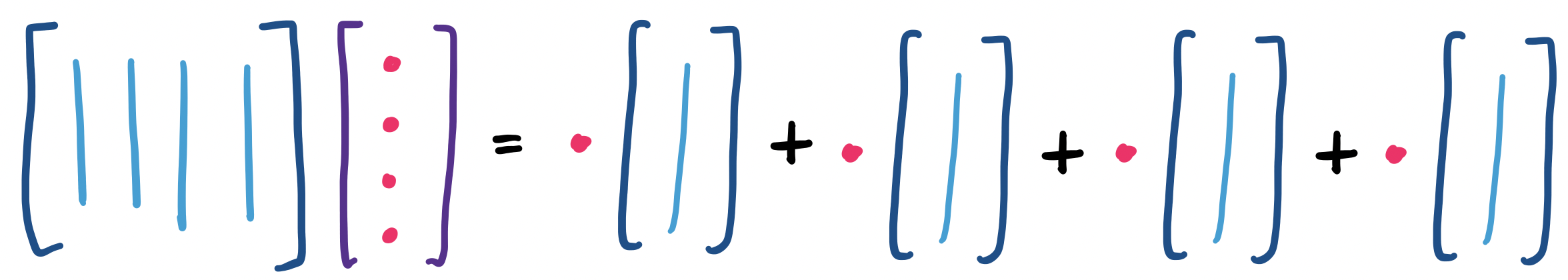
What does this mean? In a sense, we can view the vector $\mathbf v$ as encoding a linear combination of the vectors that form the columns of $A$. That is, \[ A \mathbf v = 1 \begin{bmatrix} 2 \\ -3 \end{bmatrix} + 5 \begin{bmatrix} -4 \\ 4 \end{bmatrix} = \begin{bmatrix} 2 \\ 3 \end{bmatrix} + \begin{bmatrix} -20 \\ 20 \end{bmatrix} = \begin{bmatrix} -18 \\ 17 \end{bmatrix}.\]
In other words, the product of a matrix $A$ and a vector $\mathbf v$ is a linear combination of the columns of $A$!
There is an alternative view of this product. If $b_i$ is the $i$th entry of the vector $\mathbf b = A \mathbf v$, we can get this by finding \[b_i = A_{i,1} v_1 + A_{i,2} v_2 + \cdots + A_{i,n} v_n.\]
So from above, \[ A \mathbf v = \begin{bmatrix} 2 \times 1 + -4 \times 5 \\ -3 \times 1 + 4 \times 5 \end{bmatrix} = \begin{bmatrix} -18 \\ 17 \end{bmatrix}. \]
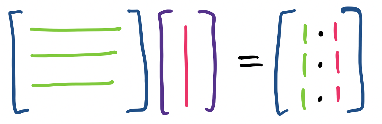
But those expressions look very familiar. Some observation can lead us to conclude that a more succinct description of this process is that we consider each row of the matrix as a vector and take its dot product with $\mathbf v$ to get the corresponding entry. A lot of people like this definition because it's very computational: it tells us how each entry is computed.
These two approaches highlight a key difference in how we view the objects that we're studying. A traditional approach will focus on computation: what are the numbers that we get out of a procedure. But what we want to do is understand the structure of the objects and the way to do this is to see how they're formed by the operations that we're interested in.
Let's generalize this.
Let $A = \begin{bmatrix}\mathbf u & \mathbf v & \mathbf w\end{bmatrix}$ be a matrix with column vectors $\mathbf u, \mathbf v, \mathbf w$. Let $\mathbf x = \begin{bmatrix}x_1 \\ x_2 \\ x_3 \end{bmatrix}$. Then \[A\mathbf x = \begin{bmatrix}\mathbf u & \mathbf v & \mathbf w\end{bmatrix} \begin{bmatrix}x_1 \\ x_2 \\ x_3 \end{bmatrix} = x_1 \mathbf u + x_2 \mathbf v + x_3 \mathbf w.\] And, \[x_1 \mathbf u + x_2 \mathbf v + x_3 \mathbf w = x_1 \begin{bmatrix}u_1 \\ u_2 \\ u_3 \end{bmatrix} + x_2 \begin{bmatrix} v_1 \\ v_2 \\ v_3 \end{bmatrix} + x_3 \begin{bmatrix} w_1 \\ w_2 \\ w_3 \end{bmatrix} = \begin{bmatrix} x_1 u_1 + x_2 v_1 + x_3 w_1 \\ x_1 u_2 + x_2 v_2 + x_3 w_2 \\ x_1 u_3 + x_2 v_3 + x_3 w_3 \end{bmatrix}.\]
We can think about this visually. First, if we view the matrix-vector product as a linear combination of the columns of the matrix, we see something like
And if we think about the product as entries that are formed from dot products of the vector with the rows of the matrix, we have
So now, it's worth thinking about what a matrix means or represents. That a matrix has rows and columns provides two immediate interpretations. One is to view the matrix as a collection of rows. This is the view that one would arrive at directly from algebra. The rows correspond to linear equations and so the matrix represents a system of linear equations.
The second is to view the matrix as a description for a collection of vectors. These vectors are linear combinations of the columns of the matrix. Of course, the system of linear equations describes the exact same set of vectors. But this is a very useful trick in math—certain problems make more sense from a particular perspective.
This idea is so important that it has a name. The linear combinations of the columns of a matrix $A$ is called the column space of $A$.
Why is this important? This view of a matrix as a description of vectors provides a window into some of the things that we try to accomplish in machine learning and data science. It's not hard to see that we can envision a matrix very plainly as a table of data, where a column represents an object and a row represents a particular attribute. This matrix is likely to be very large, so what we really want is a way to describe what's special about the matrix succinctly.
If we consider this question from the perspective of linear algebra, what we're really looking to do is find a simpler way to describe the space of vectors represented by this matrix. Equivalently, this means trying to come up with a smaller matrix that captures a lot of the same patterns as our original matrix of data.
The promise of linear algebra is that because these are all matrices, the functions or operators are all linear. Because linear algebra is pretty well understood, this means we can play around with the tools of linear algebra to come up with such an approximation instead of trying to invent all sorts of new math.
This fact is actually kind of amazing. After all, why should linear methods be sufficient for working with large data? Why is it that we don't have to stretch ourselves and go do something more complicated like use fancier polynomials? It's a good thing we don't, because it's much harder to work with more complicated mathematics, both for the people working on this stuff and in terms of the computational power required.
In this sense, we can think of $A$ as a function on vectors. Here, $A$ takes a vector $\mathbf x$ as input and produces another vector as output. Then we can think of $A$ as a description of a particular set of vectors. This is the perspective that machine learning tries to take: the learning in machine learning is about "learning" a function, or trying to come up with a good approximation of the original function.