Projections allow us to unlock a tool that answers the question of what to do when we are faced with a linear equation $A \mathbf x = \mathbf b$ with no solution. Recall that in such cases, we have a vector that lines outside of the column space of $A$. In practical terms, we have a sample that lies outside of our model for our dataset. This is not an uncommon situation so we can't just throw up our hands and give up. So what to do?
Our discussion of projections has already hinted at this: find the closest point that is in the desired subspace. What this means is that for a matrix $A$, if $\mathbf b$ is not in the column space of $A$, we want to find instead a solution for the vector in the column space of $A$ that is closest to $\mathbf b$. We already have an answer for this: it's the projection of $\mathbf b$ onto the column space of $A$!
The key here is something we mentioned offhandedly earlier: that the projection is the vector in the column space of $A$ for which the error is minimized. Here, the error is the vector $\mathbf e = \mathbf b - \mathbf p$ and the length of that error is $\|\mathbf e\|$.
Recall that by definition, we have $\mathbf p = A \mathbf{\hat x}$, so we have $\mathbf e = \mathbf b - A \mathbf{\hat x}$. By this, we have that $\|\mathbf e\| = \|\mathbf b - A \mathbf{\hat x}\|$. To minimize $\|\mathbf e\|$, we need to minimize $\|\mathbf b - A \mathbf{\hat x}\|^2$, which leads us to what you may know as the least squares approximation.
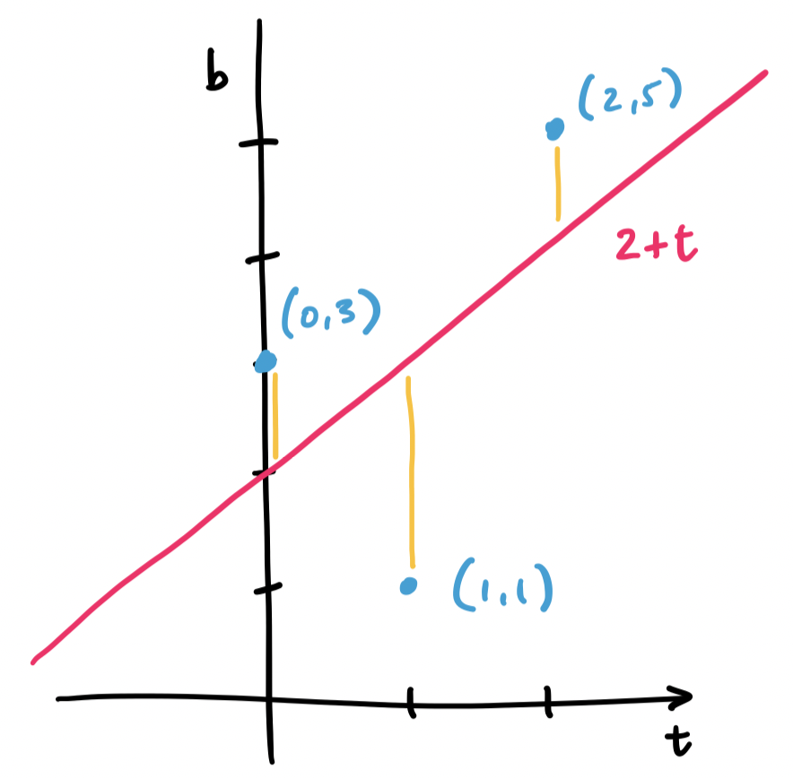
First, let's consider this problem geometrically. Consider the three points $(0,3), (1,1), (2,5)$. We want to fit a line through these points, but no single line will contain all three. Instead, we find the line that will minimize the distance to all three.
Let's consider a line $y = mx + b$, but call it instead $b = C + Dt$, since many of those variables have been used. What we have with our example is trying to solve the system of equations \begin{align*} C + D \cdot 0 &= 3 \\ C + D \cdot 1 &= 1 \\ C + D \cdot 2 &= 5 \end{align*} This gives us matrices and vectors $A = \begin{bmatrix} 1 & 0 \\ 1 & 1 \\ 1 & 2 \end{bmatrix}$, $\mathbf b = \begin{bmatrix} 3 \\ 1 \\ 5 \end{bmatrix}$, and $\mathbf x = \begin{bmatrix} C \\ D \end{bmatrix}$.
Again, we realize that $\mathbf b$ lies outside of the column space of $A$. This means that there is no solution $C$ and $D$ for our line. So we must instead find $C$ and $D$ for the closest vector that is in the column space. This is our projection, and this makes the question of finding an appropriate $\begin{bmatrix} C \\ D \end{bmatrix}$ the same question as finding $\mathbf{\hat x}$.
Since we've already done this exact example, we have that $C = 2$ and $D = 1$. This gives us the line $2 + t$, which looks like it does a pretty good job of getting close to all of our points.
Now, let's look at it in the statistical/data/machine learning sense—as linear regression. Here, we have some data:
| $t$ | $b$ |
|---|---|
| 0 | 3 |
| 1 | 1 |
| 2 | 5 |
We want to model this data by predicting $b$ given the one feature $t$. We assume that there's a linear relationship, so we try to find a linear function $b = C + Dt$. In other words, we want to figure out what the parameters $C$ and $D$ should be.
How do we figure this out? First, we recognize that generally, we're trying to define a subspace—in this case a line, but really, we can define any linear subspace we want. Then not every data point is going to be in that subspace—there will be error. So we want the subspace that minimizes the error. How do we determine this error? By taking the square of the lengths of the error vectors for our dataset—least squares.
The least squares solution for an equation $A \mathbf x = \mathbf b$ is $\mathbf{\hat x}$. That is, $\|\mathbf b - A\mathbf x\|^2$ is minimized when $\mathbf x = \mathbf{\hat x}$.
Recall that for any vector $\mathbf b$ in $\mathbb R^m$, it can be written as two vectors: one in the column of an $m \times n$ matrix $A$ and the other in the left null space of that same matrix $A$. We have been calling these $\mathbf p$, the projection of $\mathbf b$ in $\mathbf C(A)$, and $\mathbf e$, the error vector, which belongs to $\mathbf N(A^T)$.
We want to justify that this is the right choice, so we have to think about their lengths—the least squares approximation is the one that minimizes $\|A \mathbf x - \mathbf b\|$, the difference between the desired solution and our best approximation. In other words, we need to solve for $\mathbf x$ so that this quantity is minimized in the following equation: \[\|A\mathbf x - \mathbf b\|^2 = \|A \mathbf x - \mathbf p\|^2 + \|\mathbf e\|^2.\] This is the Pythagorean theorem applied to our vectors of interest. But we have an answer for this: we know that $\mathbf p = A \mathbf{\hat x}$, so choosing $\mathbf x = \mathbf{\hat x}$ makes $\|A\mathbf x-\mathbf p\|^2 = 0$. Since $\mathbf e$ is fixed, this is the best we can do, so $\mathbf{\hat x}$ is our least squares solution.
Notice that this proof rehashes a lot of the same observations we made about $\mathbf p$ and $\mathbf e$. The difference is in where we started and what we were trying to find. Before, we wanted to know how to get $\mathbf p$ while here, we're trying to show that $\mathbf{\hat x}$ minimizes $\|A \mathbf x - \mathbf b\|$. Because $\mathbf p$ is the "closest" vector in the column space of $A$ to $\mathbf b$, we end up with a lot of overlap in the two arguments.
We can generalize this to any number of points.
Let $(t_1, b_1), \dots, (t_m, b_m)$ be a set of $m$ points. The least squares approximation of a line that goes through all $m$ points is the line $b = C + Dt$, where $\begin{bmatrix} C \\ D \end{bmatrix}$ is the least squares solution to the equation \[\begin{bmatrix} m & \sum\limits_{i=1}^m t_i \\ \sum\limits_{i=1}^m t_i & \sum\limits_{i=1}^m t_i^2 \end{bmatrix} \begin{bmatrix} C \\ D \end{bmatrix} = \begin{bmatrix} \sum\limits_{i=1}^m b_i \\ \sum\limits_{i=1}^m t_ib_i \end{bmatrix}.\]
Suppose we want to fit a line to $m$ points $(t_1, b_1), \dots, (t_m, b_m)$. We would like for this line $b = C + Dt$ to satisfy $b_i = C + Dt_i$ for all of our points, but that is very unlikely. We set up our system in the same way. \[\begin{bmatrix} b_1 \\ \vdots \\ b_m \end{bmatrix} = \begin{bmatrix} 1 & t_1 \\ \vdots & \vdots \\ 1 & t_m \end{bmatrix} \begin{bmatrix} C \\ D \end{bmatrix}.\] This is our equation $\mathbf b = A \mathbf x$. This means we need to find $\mathbf{\hat x}$ by solving $A^T A \mathbf{\hat x} = A^T \mathbf b$.
Let's examine each piece. What is $A^T A$? It is the matrix \[\begin{bmatrix} 1 & \cdots & 1 \\ t_1 & \cdots & t_m \end{bmatrix} \begin{bmatrix} 1 & t_1 \\ \vdots & \vdots \\ 1 & t_m \end{bmatrix} = \begin{bmatrix} 1 \cdot 1 + \cdots + 1 \cdot 1 & 1 \cdot t_1 + \cdots + 1 \cdot t_m \\ t_1 \cdot 1 + \cdots + t_m \cdot 1 & t_1 \cdot t_1 + \cdots + t_m \cdot t_m \end{bmatrix} = \begin{bmatrix} m & \sum\limits_{i=1}^m t_i \\ \sum\limits_{i=1}^m t_i & \sum\limits_{i=1}^m t_i^2 \end{bmatrix} \] Then $A^T \mathbf b$ is \[\begin{bmatrix} 1 & \cdots & 1 \\ t_1 & \cdots & t_m \end{bmatrix} \begin{bmatrix} b_1 \\ \vdots \\ b_m \end{bmatrix} = \begin{bmatrix} 1 \cdot b_1 + \cdots + 1 \cdot b_m \\ t_1 \cdot b_1 + \cdots + t_m \cdot b_m \end{bmatrix} = \begin{bmatrix} \sum\limits_{i=1}^m b_i \\ \sum\limits_{i=1}^m t_ib_i \end{bmatrix}.\]
This is a nice shortcut—you can just apply this formula wihtout having to compute $A^TA$ or $A^T \mathbf b$ step by step.
The result is that we sort of fell into least squares, just by thinking about geometry and how to approximate solutions for cases where systems of equations are not solvable. In particular, it's the geometry, via orthogonality, that gives us the least squares part of the equation.
We've illustrated this with lines of best fit, which are just 1-dimensional spaces. The natural question is whether we can generalize this to more dimension. The answer is yes. For instance, suppose that our dataset has two features:
| $t_1$ | $t_2$ | $b$ |
|---|---|---|
| 0 | -2 | 9 |
| 1 | 3 | 23 |
| 2 | -24 | 1 |
| 3 | 13 | -5 |
| 4 | -3 | -12 |
Then the linear function we want to model would be something like $b = C + Dt_1 + Et_2$. But this linear function describes a plane, so what we'd be doing is trying to find is a plane of best fit. Then we end up with a matrix $A$ that has rows of the form $\begin{bmatrix} 1 & s_i & t_i \end{bmatrix}$ and $\mathbf{\hat x} = \begin{bmatrix} C \\ D\\ E \end{bmatrix}$. So our above data table turns into \[A = \begin{bmatrix} 1 & 0 & 2 \\ 1 & 1 & 3 \\ 1 & 2 & -24 \\ 1 & 3 & 13 \\ 1 & 4 & -3 \end{bmatrix}, \mathbf b = \begin{bmatrix} 9 \\ 23 \\ 1 \\ -5 \\ -12 \end{bmatrix}.\] It's not hard to see how we can add on more features to our model and we end up describing higher-dimensional spaces to predict our variable of interest, $b$.
In this setup, we notice that $D$ and $E$ plays the role of "weighting" the features $t_1$ and $t_2$ in the way that we talked about when we first introduced the dot product. And in fact, this is exactly what we are getting when we put everything together.
What's nice about this is how simply by assuming that there's a linear relationship in our data gives us enough bones to put together to get a model like this.
While we've oriented our subspaces, we've said nothing about their bases—only that these exist. But because bases are how we describe our subspaces, it stands to reason that our choice of basis matters. Bases over $\mathbb R^n$ are a good example: we would rather work with the standard basis than a basis of arbitrary vectors.
In this view, the right choice of basis can make the difference between an easy and an expensive computation. Right now, the biggest challenge in computing projections and least squares solutions is the computation of the inverse. As we mentioned earlier, computing the inverse is an expensive operation that we always try to avoid—this is the reason why we preferred methods like LU factorization.
One reason for why the standard basis is convenient is because the vectors are orthogonal. The other reason is that they are unit vectors—they have length 1. This leads us to the following definition.
A set of vectors $\mathbf q_1, \dots, \mathbf q_n$ is orthogonal when $\mathbf q_i \cdot \mathbf q_j = 0$ for all $i \neq j$. They are orthonormal if \[\mathbf q_i \cdot \mathbf q_j = \begin{cases} 0, & \text{if $i \neq j$, and } & \text{(orthogonal)} \\ 1, & \text{if $i = j$}. & \text{(unit vectors)} \end{cases}\] Notice that, by convention, we use $\mathbf q$ to denote orthonormal vectors.
There are two very useful observations to make here. One is that orthonormal vectors will "cancel" each other out to become zero. The other is that the same vectors will remain constant because they "combine" to make 1. This seems like a path forward to simplifying computations. Indeed, we immediately get the following.
Let $Q$ be an $m \times n$ matrix wtih orthonormal columns. Then $Q^TQ = I$. If $m = n$, then $Q^T = Q^{-1}$.
The nice properties of orthonormal vectors suggest that they would make for an ideal basis for any subspace. For instance, consider the problem of computing least squares approximations: \begin{align*} Q^TQ \mathbf{\hat x} &= Q^T \mathbf b \\ \mathbf{\hat x} &= Q^T \mathbf b & \text{since $Q^TQ = I$} \end{align*} Notice that since $Q^TQ$ disappears, we have no need to compute the inverse anymore to get $\mathbf{\hat x}$. From here, we get \[\mathbf p = Q \mathbf{\hat x} = QQ^T \mathbf b = \mathbf q_1 (\mathbf q_1^T \mathbf b) + \cdots + \mathbf q_n (\mathbf q_n^T \mathbf b),\] which greatly simplifies our computation into a series of one-dimensional projections. The projection matrix is similar: \[P = Q(Q^TQ)^{-1}Q^T = QQ^T,\] which sees the projection matrix as a sum of the projection matrices for each column.