We saw last class that for any vector space, if we have a pair of subspaces that are orthogonal complements, we can express any vector in that vector space as the sum of unique vectors from each subspace. This makes the fact that the fundamental subspaces for any given matrix are orthogonal complements very useful.
Let $A = \begin{bmatrix} 3 & 1 \\ 9 & 3 \end{bmatrix}$ and consider the vector $\begin{bmatrix} 7 \\ 9 \end{bmatrix}$. The rref of $A$ is $\begin{bmatrix} 1 & \frac 1 3 \\ 0 & 0 \end{bmatrix}$, which gives a null space spanned by $\begin{bmatrix} -\frac 1 3 \\ 1 \end{bmatrix}$. Then we can write $\begin{bmatrix} 7 \\ 9 \end{bmatrix} = \begin{bmatrix} 9 \\ 3 \end{bmatrix} + \begin{bmatrix} -2 \\ 6 \end{bmatrix}$.
Of course, this doesn't tell us how to split up our vector into these parts, onlt that we can. This brings us to the idea of projection.
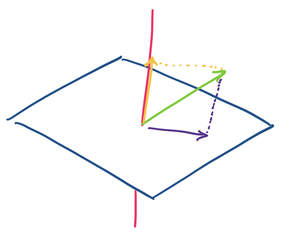
There are a few ways to think about this. The usual analogy for projection is of a light casting a shadow on a surface. The shadow is the projection of the object onto the surface, which is our subspace. We get a nice visual when we imagine this in $\mathbb R^3$.
Consider a vector $\mathbf v$ in $\mathbb R^3$. We want to consider projections on the $x,y$-plane and the $z$ axis. It's clear that if $\mathbf v = \begin{bmatrix} x \\ y \\ z \end{bmatrix}$, then our two projections are $\begin{bmatrix} x \\ y \\ 0 \end{bmatrix}$ and $\begin{bmatrix} 0 \\ 0 \\ z \end{bmatrix}$.
As usual, we can encode projections as matrices. For projection onto the $x,y$-plane, we have $\begin{bmatrix} 1 & 0 & 0 \\ 0 & 1 & 0 \\ 0 & 0 & 0 \end{bmatrix}$ and $\begin{bmatrix} 0 & 0 & 0 \\ 0 & 0 & 0 \\ 0 & 0 & 1 \end{bmatrix}$ for projection onto the $z$-axis.
We notice that this works out quite nicely because our two chosen subspaces happen to be orthogonal complements. In fact, one realizes that the proof that every vector in $\mathbb R^n$ can be written as a row space vector and a null space vector with respect to any matrix $A$ is really a proof that every vector in a vector space can be written as two vectors, one from each of two orthogonal complements—no matter what those orthogonal complments are!
This is the easy case. But what if our subspaces are not perfectly aligned with the standard axes? What we want is to generalize this for higher dimensional spaces and for subspaces that are not perfectly aligned to our standard axes.
This seems like a geometric exercise, but, projections are neither just an idea that works only in geometry nor is it just an abstract concept when we move to higher-dimensional spaces. Among a whole host of applications, one that we can imemediately discuss is how we implicitly apply the idea of projections every time we take some high-dimensional data and attempt to visualize it.
Suppose you have a record of votes for an unnamed officially nonpartisan legislature as an $m \times n$ matrix, where columns are a member's voting record and each row is the vote that was taken. The entries can be defined by \[a_{ij} = \begin{cases} -1 & \text{if member $j$ voted NO on vote $i$,} \\ 0 & \text{if member $j$ was absent for vote $i$,} \\ 1 & \text{if member $j$ voted YES on vote $i$.} \end{cases}\] This dataset is not particularly large as far as datasets go—maybe something like 50 members and maybe a couple hundred votes in one legislative session. Even something like a few hundred members is not particularly large. However, it is still too large for humans to be able to make anything of any patterns that crop up.
Since we have a nominally non-partisan chamber, one question that we can ask is whether there are any unofficial groups of members that tend to vote together. Note that thinking about the rank of the matrix alone is unlikely to give us anything useful—with so many votes and relatively few members in comparison, we have a tall, skinny matrix, so it's likely that exact rank of the matrix is close to the number of members (sort of the opposite of our Netflix recommendation system matrix). So to uncover any patterns or structure, we need to do a bit of transformation on the data. There are a few ways to do this—scoring members, or trying to plot their voting habits on some chart.
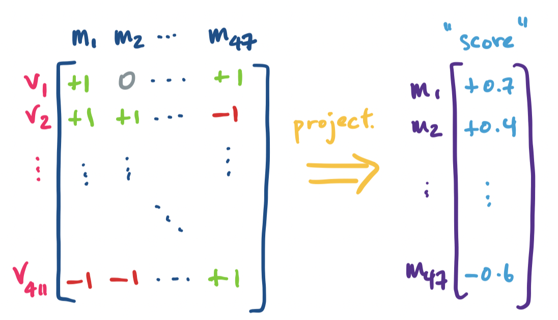
In this sense, a single numeric score is a 1-dimensional projection of our data. A graph or plot is a 2-dimensional projection, or if we get really fancy, we can get a 3-dimensional projection. In each of these cases, we are taking our high-dimensional data ($m$- or $n$-dimensional) and transforming it into a lower-dimensional space while trying to preserve certain structures, relationships, and characteristics. If our transformation is a linear transformation, we have a matrix for that transformation, and if we have a matrix, we have subspaces that we want to project things onto.
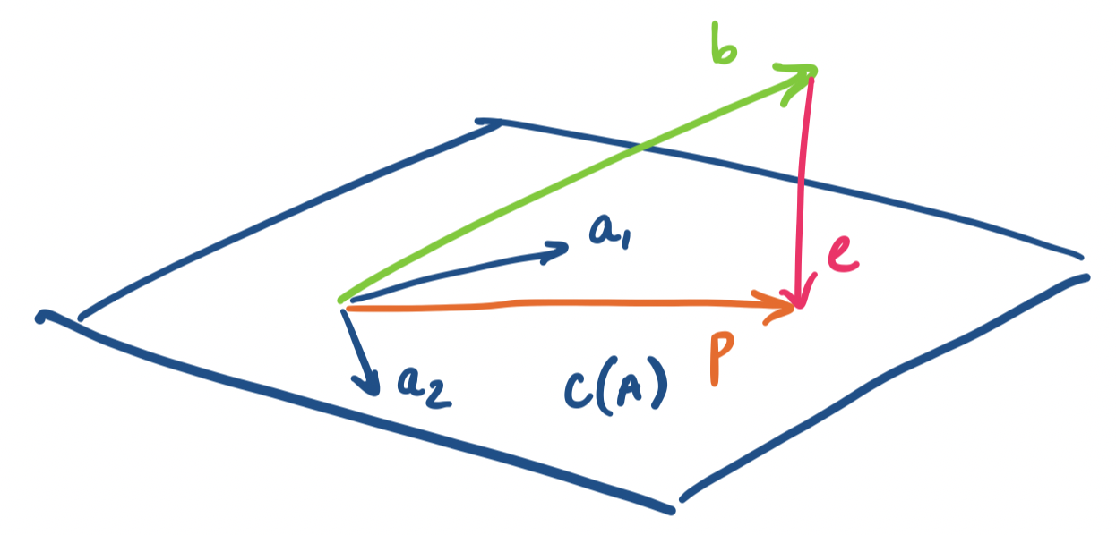
We begin with the simplest subspace to project onto: a line. Lines are defined by a single vector, which we denote by $\mathbf a$. We will project a vector $\mathbf b$ onto the line going through $\mathbf a$. The projection is called $\mathbf p$.
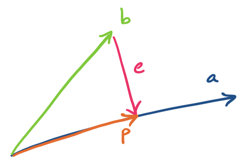
There are a few things to note here. Since $\mathbf p$ is on the line going through $\mathbf a$, it must be a scalar multiple of $a$. This gives us $\mathbf p = \mathbf{\hat x} \mathbf a$. (Notice that we're being rebels and using boldface for a scalar—this will be important when we generalize)
So how do we find $\mathbf{\hat x}$? First, we notice that we can talk about the distance between $\mathbf b$ and its projection $\mathbf p$ onto $\mathbf a$. This is called the error, and is the vector $\mathbf e = \mathbf b - \mathbf p$.
We notice that the error $\mathbf e$ is perpendicular to $\mathbf a$ (and $\mathbf p$). The claim that we're making is that this is the vector $\mathbf e$ that minimizes the distance between $\mathbf b$ and $\mathbf p$ (i.e., $\|\mathbf e\|$ is minimized). We make use of this to come up with an expression for $\mathbf{\hat x}$.
The projection $\mathbf p$ of $\mathbf b$ onto $\mathbf a$ is \[\mathbf p = \mathbf{\hat x} \mathbf a = \mathbf a \frac{\mathbf a^T \mathbf b}{\mathbf a^T \mathbf a}.\]
We have that $\mathbf p = \mathbf{\hat x} \mathbf a$ for some scalar $\mathbf{\hat x}$. We observe that $\mathbf e = \mathbf b - \mathbf{\hat x} \mathbf a$ is perpendicular to $\mathbf a$ when $\|\mathbf e\|$ is minimized. So we have \begin{align*} \mathbf a \cdot \mathbf e &= 0 \\ \mathbf a \cdot (\mathbf b - \mathbf{\hat x} \mathbf a) &= 0 \\ \mathbf a \cdot \mathbf b - \mathbf{\hat x}(\mathbf a \cdot \mathbf a) &= 0 \\ \mathbf{\hat x} &= \frac{\mathbf a \cdot \mathbf b}{\mathbf a \cdot \mathbf a} \end{align*}
In other words, $\mathbf{\hat x} = \frac{\mathbf a^T \mathbf b}{\mathbf a^T \mathbf a}$.
Let $\mathbf b = \begin{bmatrix} 1 \\ -2 \\ 1 \end{bmatrix}$. We will project $\mathbf b$ onto $\mathbf a = \begin{bmatrix} 3 \\ 1 \\ 2 \end{bmatrix}$. We need to compute $\mathbf{\hat x}$ to get $\mathbf p$. We have \[\mathbf a^T \mathbf a = 3^2 + 1^2 + 2^2 = 14\] \[\mathbf a^T \mathbf b = 3 \cdot 1 + 1 \cdot -2 + 2 \cdot 1 = 3\] This gives $\mathbf{\hat x} = \frac{3}{14}$. So $\mathbf p = \begin{bmatrix} \frac{9}{14} \\ \frac{3}{14} \\ \frac{6}{14} \end{bmatrix}$.
We can verify this by considering the other definition for $\mathbf p$, that $\mathbf e = \mathbf b - \mathbf p$. We first compute \[\mathbf e = \begin{bmatrix} 1 \\ -2 \\ 1 \end{bmatrix} - \begin{bmatrix} \frac{9}{14} \\ \frac{3}{14} \\ \frac{6}{14} \end{bmatrix} = \begin{bmatrix} \frac{5}{14} \\ -\frac{31}{14} \\ \frac{8}{14} \end{bmatrix}.\] Then \[\mathbf e \cdot \mathbf a = 3 \cdot \frac{5}{14} - \frac{31}{14} + 2 \cdot \frac{8}{14} = 0,\] as desired.
Now, we want to encode this projection as a matrix $P$. We work backwards, noting that we should have $\mathbf p = P \mathbf b$.
Let $\mathbf p$ be the projection of $\mathbf b$ on $\mathbf a$. Then $\mathbf p = P \mathbf b$, where $P = \frac{\mathbf a \mathbf a^T}{\mathbf a^T \mathbf a}$.
To get our projection matrix $P$, we simply take $\mathbf p = \mathbf a \mathbf{\hat x}$ and rearrange it. We have \begin{align*} \mathbf p &= \mathbf a \mathbf{\hat x} \\ &= \mathbf a \frac{\mathbf a^T \mathbf b}{\mathbf a^T \mathbf a} \\ &= \frac{\mathbf a \mathbf a^T}{\mathbf a^T \mathbf a} \mathbf b \\ &= \frac{1}{\mathbf a^T \mathbf a}(\mathbf a \mathbf a^T) \mathbf b \\ \end{align*}
This tells us that our projection matrix $P$ is a rank 1 matrix $\mathbf a \mathbf a^T$, that is scaled by $\mathbf a \cdot \mathbf a$.
From our earlier example, we had $\frac{1}{\mathbf a^T \mathbf a} = \frac{1}{14}$. Then we compute the rank 1 matrix \[\mathbf a \mathbf a^T = \begin{bmatrix} 9 & 3 & 6 \\ 3 & 1 & 2 \\ 6 & 2 & 4 \end{bmatrix}.\] Together, this gives us \[P = \frac{\mathbf a \mathbf a^T}{\mathbf a^T \mathbf a} = \frac{1}{14} \begin{bmatrix} 9 & 3 & 6 \\ 3 & 1 & 2 \\ 6 & 2 & 4 \end{bmatrix} = \begin{bmatrix} \frac{9}{14} & \frac{3}{14} & \frac{6}{14} \\ \frac{3}{14} & \frac{1}{14} & \frac{2}{14} \\ \frac{6}{14} & \frac{2}{14} & \frac{4}{14} \end{bmatrix}.\]
Notice that the projection matrix $P$ doesn't depend on $\mathbf b$ at all. The projection matrix is for projecting onto the line, which means that $P \mathbf d$ will give us the projection of some other vector $\mathbf d$ onto the line going through $\mathbf a$.
Now, how do we generalize this to a subspace of arbitrary dimension? Simple—just do the same thing but for each "dimension". Here, we see why we want a basis for our subspace—each basis vector represents a "direction" or dimension of the subspace. So if we want to project a vector onto the subspace, we simply metaphorically project the vector onto each line described each basis vector. Practically speaking, this means that our projection is going to be a linear combination of these basis vectors.
Let $\mathbf a_1, \dots, \mathbf a_n$ be vectors in $\mathbb R^m$ that span a subspace $S$. Then the projection of $\mathbf b$ onto $S$ is the vector $\mathbf p = \hat x_1 \mathbf a_1 + \cdots + \hat x_n \mathbf a_n$ in $S$ that is closest to $\mathbf b$. By closest, we mean that the length of the error vector $\mathbf e = \mathbf p - \mathbf b$ is minimized.
This means that we will be doing the same projection computation that we've been doing but on all the basis vectors all at once. As usual, our trick for working with multiple vectors at once is to throw all of them into a single matrix and express all the computations as a matrix product. Then it becomes clear that our $\hat x_i$'s are the components of a vector $\mathbf{\hat x}$ that describes the desired linear combination of the basis vectors.
We generalize our setting: instead of a single line defined by a vector $\mathbf a$, we project our vector onto a subspace with basis $\mathbf a_1, \dots, \mathbf a_n$. We take these basis vectors and put them together into a single matrix $A$. This means our projection will be given by $\mathbf p = A \mathbf{\hat x}$, where $\mathbf{\hat x}$ is a vector, not just a scalar.
First, we make an observation about the error vector again.
Let $\mathbf p$ be the projection of $\mathbf b$ onto a subspace with basis vectors $\mathbf a_1, \dots, \mathbf a_n$. Then the error vector $\mathbf e = \mathbf p - \mathbf b$ is perpendicular to all of the basis vectors.
Why is the error perpendicular to the subspace? Intuitively, the error vector forms a line straight "down" to the subspace—the shortest and fastest way to get from the vector $\mathbf b$ to the subspace.
This means that for each basis vector $\mathbf a_i$ for our subspace, we must have $\mathbf a_i^T (\mathbf b - \mathbf a_i \hat x_i) = 0$. Then we can apply the same reasoning as with projection to a line above, giving us \[\mathbf p_i = \mathbf a_i \hat x_i = \mathbf a_i \frac{\mathbf a_i^T \mathbf b}{\mathbf a_i^T \mathbf a_i}.\]
Now, recall that all of these basis vectors are columns of the matrix $A$. This means that:
So we take all of these vector products and instead think of them as matrix products instead: \[\begin{bmatrix} \rule[.5ex]{1.5em}{0.5pt} & \mathbf a_1^T & \rule[.5ex]{1.5em}{.5pt} \\ & \vdots & \\ \rule[.5ex]{1.5em}{0.5pt} & \mathbf a_n^T & \rule[.5ex]{1.5em}{.5pt} \end{bmatrix} \left( \begin{bmatrix} b_1 \\ \vdots \\ b_n \end{bmatrix} - \begin{bmatrix} \big\vert & & \big\vert \\ \mathbf a_1 & \cdots & \mathbf a_n \\ \big\vert & & \big\vert \end{bmatrix} \begin{bmatrix} \hat x_1 \\ \vdots \\ \hat x_n \end{bmatrix} \right) = \begin{bmatrix} 0 \\ \vdots \\ 0 \end{bmatrix}\] Or more succinctly, \[A^T(\mathbf b - A\mathbf{\hat x}) = \mathbf 0.\]
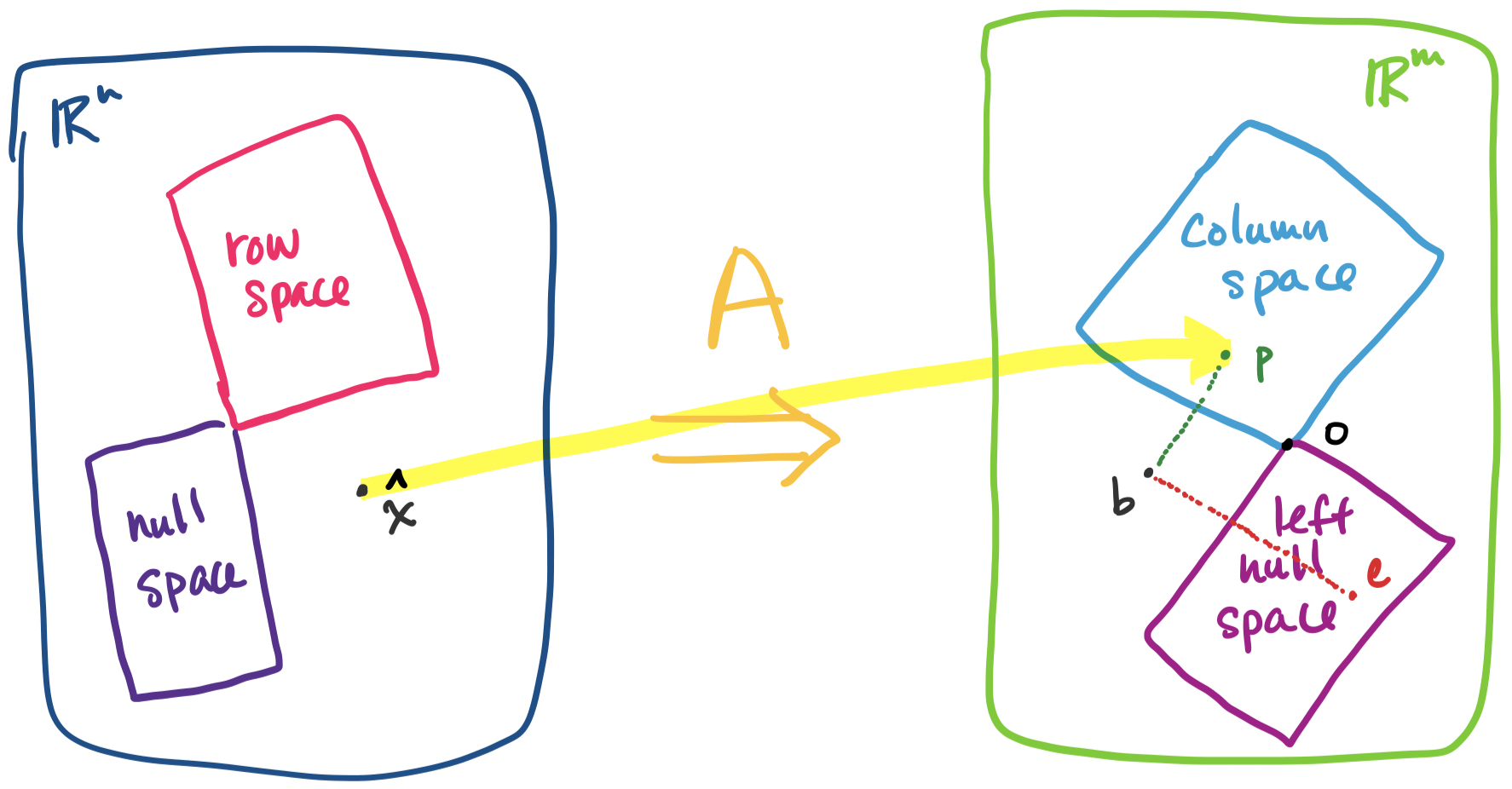
Now it becomes clear why we wrote $\mathbf a^T$ and $\mathbf{\hat x}$. We arrived at all of this geometrically, but we should take a step back and examine this closely. Recall that $\mathbf b - A \mathbf{\hat x} = \mathbf e$ by definition. So our equation above tells us \[A^T \mathbf e = \mathbf 0.\] In other words, $\mathbf e$ is in the left nullspace of $A$! This makes sense because $\mathbf e$ is orthogonal to the column space of $A$, so by orthogonal complements, this can be the only outcome.
But recall our discussion of the decomposition of $\mathbf x = \mathbf x_r + \mathbf x_n$ where $\mathbf x$ is any vector in $\mathbb R^n$, $\mathbf x_r$ is a row space vector, and $\mathbf x_n$ is a null space vector. We have a similar outcome here: $\mathbf b = \mathbf p + \mathbf e$, where $\mathbf b$ is any vector in $\mathbb R^m$, $\mathbf p$ is a vector in the column space, and $\mathbf e$ is a vector in the left null space. Everything fits together.