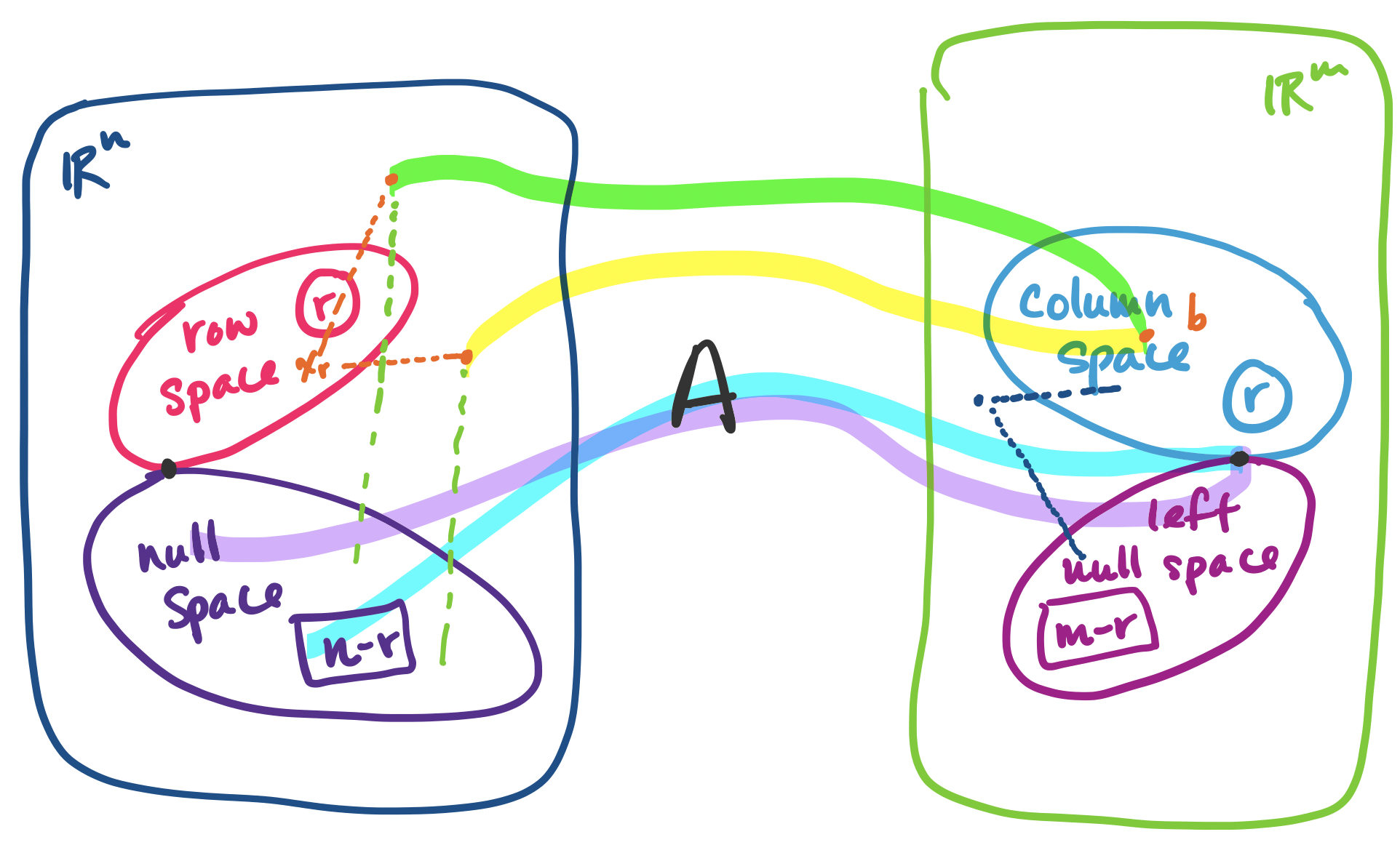
For any $m \times n$ matrix $A$ of rank $r$, we now have the following picture.
One of the intriguing suggestions of this result is that a solution to $A \mathbf x = \mathbf b$ may be written as a vector $\mathbf x = \mathbf x_r + \mathbf x_n$—that is, every vector $\mathbf b$ in the column space of $A$ is associated with some vector $\mathbf x_r$ in the row space of $A$. (Note: $\mathbf x_r$ is not $\mathbf x_p$, the particular solution) What this would say is that there's an even clearer partitioning of our data than we may have originally believed.
If $A \mathbf x = \mathbf b$ has a solution, then there is exactly one solution $\mathbf x$ that belongs to the null space.
Again, note that this is not the particular solution. But why does thinking about subspaces help us see this is true? Suppose that there were another vector $\mathbf y$ from the row space such that $A \mathbf y = \mathbf b$. Then we have $A \mathbf x - A \mathbf y = A (\mathbf x - \mathbf y) = \mathbf 0$.
Since we said that both $\mathbf x$ and $\mathbf y$ are in the row space of $A$ and the row space is a subspace, this means that $\mathbf x - \mathbf y$ is also a vector in the row space. But since $A(\mathbf x - \mathbf y) = \mathbf 0$, $\mathbf x - \mathbf y$ is a vector in the null space. But the only vector in both the row space and the null space can only be $\mathbf 0$. So this tells us $\mathbf x = \mathbf y$.
How this $\mathbf x_r$ interacts with vectors $\mathbf x_n$ in the nullspace is something we'll start talking about today. But there's more: this suggests that every vector in $\mathbb R^n$ can be expressed this way. And if this is true, we can say the same for vectors in $\mathbb R^m$: every vector in $\mathbb R^m$ can be written as a vector from the column space of $A$ together with a vector from the left null space of $A$. This is the beginnings of the strategy to being able to say something about how to deal with the question of $A \mathbf x = \mathbf b$ when there is no solution.
So far, we've dealt with vectors that are firmly located within our subspaces of interest—when we have solutions to $A \mathbf x = \mathbf b$. But what if the equation is unsolvable and $\mathbf b$ isn't in our column space?
From the perspective of data, this is a sample that lies outside of the space defined by some description of our dataset. What can we say about it? Well, we can determine which "point" is "closest" to it. However, this requires orienting our data and all of the subspaces we've been dealing with. After all, what does it mean for a vector to be "close" to some point of a vector space?
An important notion and tool for doing this orientation is the notion of orthogonality. Up until now, we've been dealing with sets of vectors like spanning sets and bases without thinking about their orientation—as long as they are independent and all point in a "new" direction, we've been happy. But a natural orientation is to have our basis vectors be orthogonal with each other—this property makes visualizing and computing with these objects much more convenient.
This is where a lot of the geometric notions we briefly introduced start coming into play. Recall the following properties and definitions.
Note the third point: transpose notation now lets us write dot products $\mathbf u \cdot \mathbf v$ as $\mathbf u^T \mathbf v$, a common idiom that we'll begin seeing a lot. This actually isn't that strange—it's exactly what we do when we compute matrix products for each entry: every entry of $AB$ is the dot product of a row of $A$ with a column of $B$. We'll see it's this exact operation that makes it a nice way to generalize ideas from vectors to matrices.
Something that's often done in math is "lifting" a definition for a single item to a set of items. For instance, we have a definition for orthogonality of two vectors: they're at a 90° angle and their dot product is 0. We can then "lift" this definition to vector spaces.
Two subspaces $U$ and $V$ are orthogonal if every vector $\mathbf u$ in $U$ is orthogonal to every vector $\mathbf v$ in $V$. That is, $\mathbf u^T \mathbf v = 0$ for all $\mathbf u$ in $U$ and $\mathbf v$ in $V$.
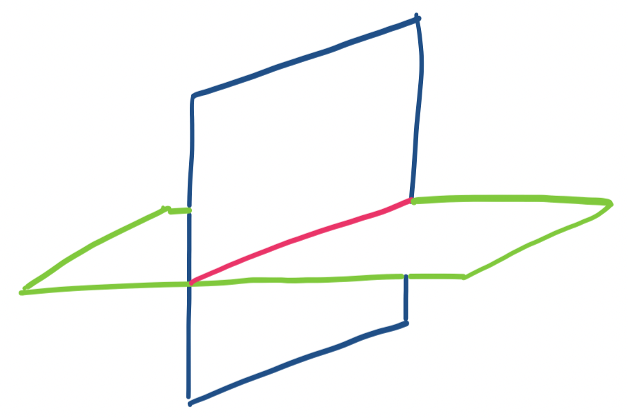
Consider the intersection of two planes at a 90° angle, like the walls of a room. These seem like they are orthogonal subspaces, but they aren't. The definition of orthogonality says that every vector in one subspace must be orthogonal to every vector in the other one. However, our two planes would intersect along a line The problem with this is that all the vectors at that intersection belong to both subspaces. This breaks our definition because it means there are a set of vectors that need to be orthogonal to themselves, which is impossible.
Note that by this definition, this means the only vector that can belong to two orthogonal subspaces is the zero vector. Our definition of orthogonality says that two vectors are orthogonal as long as their dot product is zero. The only vector for which that is true when taking a dot product with itself is $\mathbf 0$.
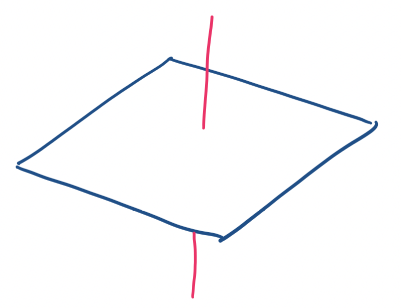
Consider the $x,y$-plane and the $z$ axis in $\mathbb R^3$. These are orthogonal subspaces: every vector on the $z$ axis is orthogonal to the $x,y$-plane and vice-versa.
These two examples suggest an interesting property: two subspaces can't be orthogonal if their dimensions together exceed the dimensions of the vector space they're in. In the first example, the planes were both 2-dimensional in a 3-dimensional space. In the second example, a line is 1-dimensional and the plane is 2-dimensional, which fits inside the 3-dimensional space.
With this, we can proceed to our big result.
Let $A$ be an $m \times n$ matrix. The null space of $A$ is orthogonal to the row space of $A$.
The null space is the set of all vectors $\mathbf x$ that satisfy $A \mathbf x = \mathbf 0$. So if $\mathbf a_1, \dots, \mathbf a_m$ are the rows of $A$, we have that $\mathbf a_i^T \mathbf x = 0$ for every $i$. By definition, this means that every row vector of $A$ is orthogonal to $\mathbf x$.
Since $\mathbf x$ is orthogonal to every row of $A$, it is orthogonal to any vector that is a linear combination of rows of $A$. So $\mathbf x$ is orthogonal to every vector in the row space of $A$. But $\mathbf x$ was any vector from the null space, so every vector in the null space of $A$ is orthogonal to every vector in the row space of $A$. So the null space is orthogonal to the row space.
Let $A = \begin{bmatrix} 1 & 3 & 1 \\ 1 & 9 & 3 \end{bmatrix}$. Then $\begin{bmatrix} 0 \\ -1 \\ 3 \end{bmatrix}$ is perpendicular to the rows of $A$. We see also that this means that it must be in the null space of $A$.
There's another way of writing this by focusing on vectors.
Take a vector $\mathbf x$ from the null space of $A$. Now, take a vector from the row space of $A$. Recall that the row space of $A$ is the column space of $A^T$. So a vector from the row space can be written as a vector $A^T \mathbf y$ for some $\mathbf y$ in $\mathbb R^n$. We get \[\mathbf x \cdot A^T \mathbf y = x^T (A^T \mathbf y) = (\mathbf x^T A^T) \mathbf y = (A\mathbf x)^T \mathbf y = \mathbf 0^T \mathbf y = \mathbf 0 \cdot \mathbf y = 0.\] So $\mathbf x$ is a vector that is perpendicular to the vector $A^T \mathbf y$. So every vector in the null space of $A$ is perpendicular to every vector in the row space of $A$.
What is nice about this is that if we take $A$ and transpose it to $A^T$, we can do the exact same proof to get the following:
Let $A$ be an $m \times n$ matrix. The left null space of $A$ is orthogonal to the column space of $A$.
This quickly brought us to the second part of the Fundamental Theorem of Linear Algebra. First, we define the following notion.
Let $V$ be a subspace of a vector space $W$. The orthogonal complement $V^{\bot}$ of $V$ is the subspace of all vectors perpendicular to a vector in $V$. Furthermore, $\dim V + \dim V^{\bot} = \dim W$.
It is possible to have two very small orthogonal subspaces. For example, two lines can be orthogonal in $\mathbb R^6$. However, these would not be orthogonal complements. The definition says that two subspaces that are orthogonal complements will have dimensions that add to the full dimension of the vector space.
In fact, two spaces being orthogonal complements is a very strong relationship. Suppose we have two subspaces $V$ and $W$. If we know that a vector $\mathbf u$ is perpendicular to some basis for $V$, then we know it must belong to $W$.
Let $A$ be an $m \times n$ matrix. Then
This result allows us to revisit an idea we discussed earlier: the fact that for the linear equation $A \mathbf x = \mathbf b$, every solution $\mathbf x$ can be described as a vector $\mathbf x = \mathbf x_r + \mathbf x_n$, where $\mathbf x_r$ is in the row space of $A$ and unique for $\mathbf b$ and $\mathbf x_n$ is a vector from the null space of $A$.
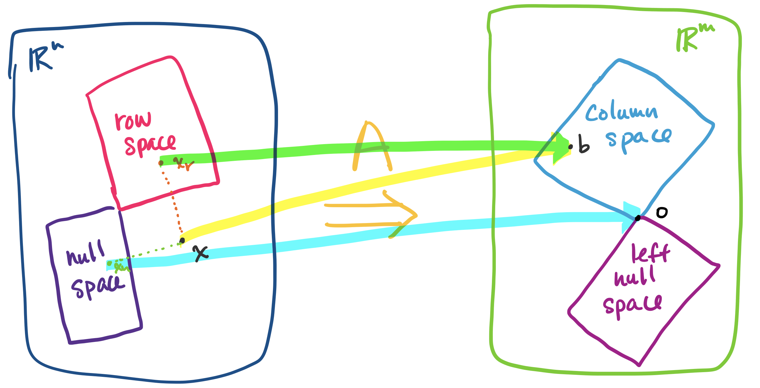
How does this help us? Consider the example of $A$ as an operation that transform a vector $\mathbf x$ in $\mathbb R^n$ into a vector $\mathbf b$ in $\mathbb R^m$. When this occurs, some part of the information in this vector gets "lost" or "flattened"—this is the part of the vector in the null space. However, up until now, we haven't had a way to talk about how to 'get' this part of the vector.
It is orthogonality, which describes how the null space of a matrix is oriented with respect to its row space, that will give us the tools to do so.
Let $A$ be an $m \times n$ matrix and let $\mathbf x$ be a vector in $\mathbb R^n$. Then it can be written as the sum of two vectors $\mathbf x_r + \mathbf x_n$, where $\mathbf x_r$ is in the row space of $A$ and $\mathbf x_n$ is in the null space of $A$.
Consider a basis $\mathbf u_1, \dots, \mathbf u_r$ for the row space of $A$ and a basis $\mathbf v_1, \dots, \mathbf v_{n-r}$ for the null space of $A$. A basis for the row space has $r$ vectors, where $r$ is the rank of $A$, and a basis for the null space of $A$ has $n-r$ vectors. Therefore, we have $n$ vectors in total.
Since each set of vectors is a basis, each set is linearly independent. Since the two subspaces are orthogonal to each other, all of the vectors are linearly independent. Since our set of $n$ vectors is linearly independent, they must span $\mathbb R^n$. Therefore, they form a basis for $\mathbb R^n$.
Since the bases for the row and null spaces forms a basis for $\mathbb R^n$, every vector $\mathbf x$ can be written as a linear combination of these basis vectors, \[\mathbf x = a_1 \mathbf u_1 + \cdots a_r \mathbf u_r + b_1 \mathbf v_1 + \cdots + b_{n-r} \mathbf v_{n-r}.\] Then by grouping the terms, we can write $\mathbf x$ as \begin{align*} \mathbf x &= (a_1 \mathbf u_1 + \cdots a_r \mathbf u_r) + (b_1 \mathbf v_1 + \cdots + b_{n-r} \mathbf v_{n-r}) \\ &= \mathbf x_r + \mathbf x_n \end{align*}
If you look at the above proof carefully, you'll notice that we never actually use the fact that we have the row space and the null space of a matrix. The only way we use this information is to conclude that they are orthogonal complements—that they have the right dimensions and orientation with respect to each other. So in fact, we could replace "row space" and "null space" with any two subspaces which are orthogonal complements and use the same proof. This means that we can actually say something stronger.
Let $U$ and $V$ be subspaces of $\mathbb R^n$ that are orthogonal complements and let $\mathbf x$ be a vector in $\mathbb R^n$. Then $\mathbf x$ can be written as the sum of two vectors $\mathbf u + \mathbf v$, where $\mathbf u$ is a vector in $U$ and $\mathbf v$ is a vector in $V$.
If we proved this first, we could get that every vector in $\mathbb R^n$ can be written as a vector from the row space and a vector from the null space. Then it's not hard to see that we also have that every vector in $\mathbb R^m$ can be written as a vector from the column space and a vector from the left null space.