Why does dimension matter? It's one of the things that ties together the subspaces of a matrix. We've seen a number of subspaces associated with any given $m \times n$ matrix $A$ of rank $r$. There are the obvious ones:
We saw a not-as-obvious one:
But this leads to another possible subspace: what if we play the same trick as with the row space and think of the null space associated with $A^T$? This is called the left nullspace of $A$.
The left nullspace of an $m \times n$ matrix $A$ is the set of vectors that satisfy $A^T \mathbf y = \mathbf 0$. It is a subspace of $\mathbb R^m$.
Why is this called the left nullspace of $A$? First, let's introduce a notational trick. We are used to viewing vectors as vertical columns. But what if we treat a vector in $\mathbb R^n$ as an $n \times 1$ matrix? We get the following.
Let $\mathbf u$ and $\mathbf v$ be vectors in $\mathbb R^n$. Then $\mathbf u^T \mathbf v = \mathbf u \cdot \mathbf v$.
This is a consequence of matrix multiplication. But this notational idiom becomes surprisingly useful in the following weeks.
Using this, we can rewrite the equation $A^T \mathbf y = \mathbf 0$ in terms of $A$ as $\mathbf y^T A = \mathbf 0$. Since $A^T$ is a matrix, it's clear that it has a nullspace, so we can carry out the same proof to find that the left nullspace is a subspace. We will soon see why this subspace is important.
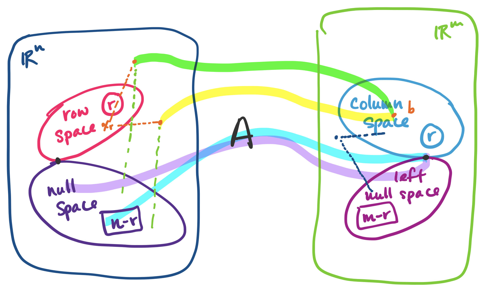
But first, let's see where we're headed. Ultimately, we will see the following: if $A$ is an $m \times n$ matrix of rank $r$, then
| Name | Notation | Subspace of | Dimension |
|---|---|---|---|
| row space | $\mathbf C(A^T)$ | $\mathbb R^n$ | $r$ |
| column space | $\mathbf C(A)$ | $\mathbb R^m$ | $r$ |
| null space | $\mathbf N(A)$ | $\mathbb R^n$ | $n-r$ |
| left null space | $\mathbf N(A^T)$ | $\mathbb R^m$ | $m-r$ |
As we've done before, the key to identifying the subspaces is by taking $A$ and transforming it into its row-reduced echelon form $R$. We'll use an example to illustrate this. Let $R = \begin{bmatrix} 1 & 3 & 1 & 0 & 9 \\ 0 & 0 & 0 & 1 & 3 \\ 0 & 0 & 0 & 0 & 0 \end{bmatrix}$. We can see that $R$ is a $3 \times 5$ matrix with rank $r = 2$.
The row space of $R$ has dimension $r$, the rank of $R$. The nonzero rows of $R$ form a basis for the row space of $R$.
In this example, $r = 2$ and there are two nonzero rows. The nonzero rows form a basis for the row space—they are independent since each row has a 1 in the pivot columns and there is no way to combine rows to get those entries.
The column space of $R$ has dimension $r$, the rank of $R$. The pivot columns of $R$ form a basis for the column space of $R$.
In this example $r = 2$ and there are two pivot columns. These pivot columns form a basis for the column space of $R$ (it's pretty clear, since togther, they form $I$).
The null space of $R$ has dimension $n-r$. The special solutions for $R \mathbf x = \mathbf 0$ form a basis for the null space of $R$.
In this example, $R$ has $5-2 = 3$ free variables, so there are three vectors in the special solutions to $R \mathbf x = \mathbf 0$, one for each free variable. They are \[\begin{bmatrix} -3 \\ 1 \\ 0 \\ 0 \\ 0 \end{bmatrix}, \begin{bmatrix} -1 \\ 0 \\ 1 \\ 0 \\ 0 \end{bmatrix}, \begin{bmatrix} -9 \\ 0 \\ 0 \\ -3 \\ 1 \end{bmatrix}.\] We observe that the special solution vectors are independent—there's a 1 in each spot corresponding to the location of the free variable and 0 in the other vectors in the same spot. So the special solutions form a basis for the null space.
The left null space of $R$ has dimension $m-r$.
The left null space of a matrix $A$ is found by finding the special solutions for $A^T$. Since we're dealing $R$, a matrix in rref, solving for its left nullspace is actually quite simple. We first see that we have \[R^T = \begin{bmatrix} 1 & 0 & 0 \\ 3 & 0 & 0 \\ 1 & 0 & 0 \\ 0 & 1 & 0 \\ 9 & 3 & 0 \end{bmatrix}.\] Since we know the rows of $R$ are independent, we can easily tell that the row-reduced echelon form of $R^T$ will be \[\begin{bmatrix} 1 & 0 & 0 \\ 0 & 1 & 0 \\ 0 & 0 & 0 \\0 & 0 & 0 \\0 & 0 & 0 \end{bmatrix}.\] In this case, the null space consists of all vectors $\begin{bmatrix} 0 \\ 0 \\ x_3 \end{bmatrix}$, so an easy basis for it is $\begin{bmatrix} 0 \\ 0 \\ 1 \end{bmatrix}$. This verifies that the dimension of the left null space of $R$ is $3-2=1$.
With this, we have covered all the subspaces for $R$. But the row-reduced echelon form matrix $R$ is shared by many matrices. So we need to take these results and connect them to the respective spaces of $A$.
The row space of $A$ is the row space of $R$.
To see this, we observe that $R$ is computed from $A$ via elimination. But elimnination involves either a permutation of the rows (i.e. a linear combination of the rows of $A$), scaling of rows (i.e. a linear combination of the rows of $A$), or subtracting multiples of one row from another (i.e. a linear combination of the rows of $A$). So because all of our operations are linear combinations of rows from the same row space, we have not changed the row space of the matrix at all.
As a corollary, because the row space of $A$ and $R$ is the same, this means that the dimension of the row space of $A$ and the basis that was computed for the row space of $R$ can be used for the row space of $A$.
The dimension of the column space of $A$ is the dimension of the column space of $R$.
Unfortunately, it is not the case that the column space of $R$ is the same as the column space of $A$—only their dimensions are the same. Consider the following example.
Let $A = \begin{bmatrix} 1 & 3 & 1 & 0 & 9 \\ 0 & 0 & 0 & 1 & 3 \\ 0 & 0 & 0 & 2 & 6 \end{bmatrix}$. Its rref is $R$. However, $\begin{bmatrix} 9 \\ 3 \\ 6 \end{bmatrix}$ is in the column space of $A$, but not in the column space of $R$.
The key difference is that $A$ has nonzero entries in the final row, but $R$ does not. This means the column spaces of the two matrices can't be the same.
So what can we say about the connection between the columns of $A$ and the columns of $R$? Intuitively, when we take combinations of rows of $A$, we are not changing anything about the positions of the columns of $A$ and they interact with each other in the same ways. Recall that we can represent the row elimnination operations as a matrix, say $E$. Then we have \begin{align*} A \mathbf x &= \mathbf 0 \\ EA \mathbf x &= E\mathbf 0 \\ R \mathbf x &= \mathbf 0 \end{align*} This tells us two things: the same combinations of columns in the same positions, specified by $\mathbf x$, gives us $\mathbf 0$. This means that whether a column was independent or not didn't change. This gives us our result: the dimension of the column space of $A$ is the same as that of $R$.
The second thing this tells us that the null space of $A$ and the null space of $R$ are the same.
The null space of $A$ is the null space of $R$.
Technically, there is one more step to take here, since all we've shown is that every vector in the null space of $A$ is in the null space of $R$. To go in reverse, we recall that elimination matrices are invertible, even in their expanded row-reduction form. We take advantage of that to get the following: \begin{align*} R \mathbf x &= \mathbf 0 \\ E^{-1}R \mathbf x &= E^{-1}\mathbf 0 \\ E^{-1}EA \mathbf x &= \mathbf 0 \\ A \mathbf x &= \mathbf 0 \end{align*} Since the null spaces of the two matrices are the same, we get our result that the dimension of the null space of $A$ is $n-r$ for free.
The dimension of the null space of $A$ is the dimension of the null space of $R$.
This comes by treating $A^T$ as a matrix and going through our previous arguments. In this case, $A^T$ has $n$ rows and $m$ columns. We know that the dimensions of its row space and column space are $r$. Then we can conclude that its null space must have dimension $m-r$.
Put together, these facts about the dimensions of the fundamental subspaces forms the first part of what the textbook calls the "Fundamental Theorem of Linear Algebra".
Let $A$ be an $m \times n$ matrix of rank $r$.
This is only part 1, which connects the dimensions of the subspaces. This will allow us to work towards a bigger goal: being able to orient these subspaces with each other. We can begin to see something like this when we think about our complete solution.