The reappearance of $A = CR$ is an opportune time to revisit some ideas that we planted at the beginning of the quarter. Abstractly, we understand this to mean that $C$ is the set of independent columns and $R$ being the set of linear combinations of those columns. From a "data" perspective, we can view $C$ as being representative profiles and $R$ as a set of weights for these profiles that correspond to particular accounts. \[\begin{bmatrix} \bigg\vert & \bigg\vert & & \bigg\vert \\ \mathbf c_1 & \mathbf c_2 & \dots & \mathbf c_m \\ \bigg\vert & \bigg\vert & & \bigg\vert \\\end{bmatrix} \begin{bmatrix} \rule[0.5ex]{3em}{0.5pt} & \mathbf r_1 & \rule[0.5ex]{3em}{0.5pt} \\ \rule[0.5ex]{3em}{0.5pt} & \mathbf r_2 & \rule[0.5ex]{3em}{0.5pt} \\ & \vdots & \\ \rule[0.5ex]{3em}{0.5pt} & \mathbf r_n & \rule[0.5ex]{3em}{0.5pt} \\ \end{bmatrix}\]
There's an obvious connection to subspaces here: all the accounts are ultimately represented in the column space as a combination of the representative profiles. However, it's not quite as simple as saying that $C$ contains everything we need to know—it's the combination of $C$ and $R$ that makes our data meaningful. We saw in a homework that the column space of $AB$ is contained in the column space of $A$, but this doesn't mean they're the same thing—the column space of $AB$ can be smaller than the column space of $A$.
But we can also view things from the perspective of the row space. Recall that each row can be viewed as an item (a movie, a book, etc.) and the row contains all of the scores or sentiment of the users reviewing that item. In this case, we can view $R$ as containing the analogous "representative profiles" of the items.
So what does the null space tell us? Recall that when we take $A \mathbf x$, the vector $\mathbf x$ encodes a series of weights, just like columns of $R$ does. If $A$ is invertible, its columns are independent and every $\mathbf x$ gets mapped to a unique vector. This is what we have been "solving" for. But the fact that every set of weights gives us something different may not be that interesting—it doesn't tell us much about what's similar to it. This is why this case is rare—$n$ equations for $n$ variables just tells us that everything is unique.
But if $A \mathbf x = \mathbf b$ doesn't have a unique solution, linear algebra tells us that $A$ has dependent columns because there are more columns than rows. One way to think about this is that we are taking something with a lot of information ($n$ measurements) and turning it into something with less information ($m$ measurements). Since you can represent and differentiate more things with $n$ measurements than $m$ measurements, you'll inevitably get natural groupings of data.
What the null space tells us is what parts of the data get flattened away—two vectors $\mathbf u$ and $\mathbf v$ give us $A \mathbf u = A \mathbf v = \mathbf b$. And since it's a subspace, we have the benefit of taking advantage of the structure: we know that there are only a certain number of representative items and that we can rely on linear combinations to describe the whole null space.
This ability to describe all vectors in the null space now lets us describe all solutions to the linear equation $A \mathbf x = \mathbf b$. We proceed with elimination again, but this time we need to make sure that we are also applying our elimination operations on the vector $\mathbf b$. The easiest way to do this is to treat the entire system as one matrix $\begin{bmatrix} A & \mathbf b \end{bmatrix}$.
Consider $A \mathbf x = \mathbf b$ with $A = \begin{bmatrix} 1 & 3 & 0 & 1 \\ 0 & 0 & 1 & 5 \\ 2 & 6 & 1 & 7 \end{bmatrix}$ and $\mathbf b = \begin{bmatrix} 2 \\ 3 \\ 7 \end{bmatrix}$. We need to perform elimination on this system and this time, we'll make sure to explicitly include $\mathbf b$. Thus we have \[\begin{bmatrix} 1 & 3 & 0 & 1 & 2 \\ 0 & 0 & 1 & 5 & 3 \\ 2 & 6 & 1 & 7 & 7 \end{bmatrix} \xrightarrow{(3) - 2 \times (1)} \begin{bmatrix} 1 & 3 & 0 & 1 & 2 \\ 0 & 0 & 1 & 5 & 3 \\ 0 & 0 & 1 & 5 & 3 \end{bmatrix} \xrightarrow{(3) - (2)} \begin{bmatrix} 1 & 3 & 0 & 1 & 2 \\ 0 & 0 & 1 & 5 & 3 \\ 0 & 0 & 0 & 0 & 0 \end{bmatrix} \] Now, to solve $A \mathbf x = \mathbf b$, we solve for $\mathbf x$ in the reduced equation $\mathbf R \mathbf x = \mathbf d$, where $\mathbf R$ is our matrix in RREF and $\mathbf d = \begin{bmatrix} 2 \\ 3 \\ 0 \end{bmatrix}$.
The fact that our augmented matrix has a row of zeros at the bottom turns out to be important—it indicates that our system is actually solvable. Why? Suppose that after row reduction we instead had a row that looked like $\begin{bmatrix} 0 & 0 & 0 & 0 & 2 \end{bmatrix}$. This is the equation $0 = 2$, which is never true!
We know already that not every system of linear equations is going to be solvable when we don't have an invertible matrix. So how do we know which vectors $\mathbf b$ do have solutions? The hint is to look at what happens after row reduction: \[\begin{bmatrix} 1 & 3 & 0 & 1 & b_1 \\ 0 & 0 & 1 & 5 & b_2 \\ 2 & 6 & 1 & 7 & b_3 \end{bmatrix} \xrightarrow{(3) - 2 \times (1)} \begin{bmatrix} 1 & 3 & 0 & 1 & b_1 \\ 0 & 0 & 1 & 5 & b_2 \\ 0 & 0 & 1 & 5 & b_3 - 2b_1 \end{bmatrix} \xrightarrow{(3) - (2)} \begin{bmatrix} 1 & 3 & 0 & 1 & b_1 \\ 0 & 0 & 1 & 5 & b_2 \\ 0 & 0 & 0 & 0 & b_3 - 2b_1 - b_2 \end{bmatrix} \] This tells us that any vector $\mathbf b$ that is solvable must have $-2b_1 - b_2 + b_3 = 0$, or $b_3 = 2b_1 + b_2$. And because we know that $A \mathbf x = \mathbf b$ is solvable only when $\mathbf b$ is in the column space of $A$, this also tells us which vectors are in the column space of $A$.
Recall that with a rectangular matrix, we can no longer guarantee that our system has a single solution since rectangular matrices cannot be inverted. Indeed, we might see situations where we have an unsolvable system. What do our matrices look like in this case? We saw last time that this occurs when the row-reduced echelon form matrices have rows of zeros that correspond to unsolvable equations—$0x_1 + \cdots + 0x_n = k$ for some $k \neq 0$.
Once we know whether our linear equation is solvable, we can try to find a solution. Of course, since we're dealing with rectangular matrices, we have possible infinitely many solutions. As with the strategy for solving $A \mathbf x = \mathbf 0$, the first step is to find some solution at all. The easiest way to do this is to set the free variables to 0. We can do this because they are free variables—we have the choice to set them and find an associated solution.
Consider the equation $R \mathbf x = \mathbf d$ with $R = \begin{bmatrix} 1 & 3 & 0 & 1 \\ 0 & 0 & 1 & 5 \\ 0 & 0 & 0 & 0 \end{bmatrix}$ and $\mathbf d = \begin{bmatrix} 2 \\ 3 \\ 0 \end{bmatrix}$. This gives us the system of equations \begin{align*} x_1 + 3 x_2 + x_4 &= 2 \\ x_3 + 5x_4 &= 3 \\ \end{align*} Since the pivots are $x_1$ and $x_3$, we set the free variables $x_2 = x_4 = 0$. This gives us $x_1 = 2$ and $x_3 = 3$ and we arrive at our solution $\mathbf x = \begin{bmatrix} 2 \\ 0 \\ 3 \\ 0 \end{bmatrix}$.
We call such a solution $\mathbf x_p$ a particular solution. Once we have this, we use the fact that $A\mathbf x_p + \mathbf 0 = A(\mathbf x_p + \mathbf u)$, where $A \mathbf u = \mathbf 0$. Again, we recall that if $A$ is invertible, then the only choice for $\mathbf u$ is $\mathbf 0$ itself. However, when $A$ has dependent columns, there are more vectors that give us $\mathbf 0$. Luckily, we know how to find these vectors.
We previously saw that the null space of $R = \begin{bmatrix} 1 & 3 & 0 & 1 \\ 0 & 0 & 1 & 5 \\ 0 & 0 & 0 & 0 \end{bmatrix}$ is spanned by its special solutions $\mathbf s_1 = \begin{bmatrix} -3 \\ 1 \\ 0 \\ 0 \end{bmatrix}$ and $\mathbf s_2 = \begin{bmatrix} -1 \\ 0 \\ -5 \\ 1 \end{bmatrix}$. Recall that $\mathbf s_1$ is the special solution with $x_2 = 1$ and $x_4 = 0$ and $\mathbf s_2$ is the special solution with $x_2 = 0$ and $x_4 = 1$. This means our complete solution, which describes all possible solutions of $R \mathbf x = \mathbf d$ can be written: \[\mathbf x_p + \mathbf x_n = \begin{bmatrix} 2 \\ 0 \\ 3 \\ 0 \end{bmatrix} + \left( x_2 \begin{bmatrix} -3 \\ 1 \\ 0 \\ 0 \end{bmatrix} + x_4 \begin{bmatrix} -1 \\ 0 \\ -5 \\ 1 \end{bmatrix} \right)\]
The idea is this: every solution that satisfies $A \mathbf x = \mathbf b$ can be described as a vector $\mathbf x = \mathbf x_p + \mathbf x_n$, where $\mathbf x_p$ is a particular solution and $\mathbf x_n$ is a vector from the null space of $A$. To describe $\mathbf x_n$, we find the special solutions for $A \mathbf x = \mathbf 0$.
Note that this is true for all matrices $A$. It just so happens that when $A$ is invertible, the only vector in the null space of $A$ is $\mathbf 0$, so we always have $\mathbf x_n = \mathbf 0$ in such cases.
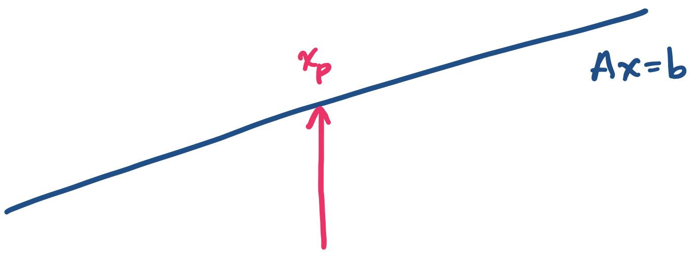
We can try to develop an intuition for what this process does by imagining this geometrically. Since we have a space of infinitely many solutions, we can think of it as a line or a plane (or if you prefer, some higher-dimensional space). Finding $\mathbf x_p$ finds one point in this space.
So how do we get to the other points? First, let's think about the null space—what does it look like? It turns out the null space is parallel to our solution space. Why is that? Consider the two equations $A \mathbf x = \mathbf b$ and $A \mathbf x = \mathbf 0$. This suggests that we have the same "space" but it's "shifted" by $\mathbf b$.
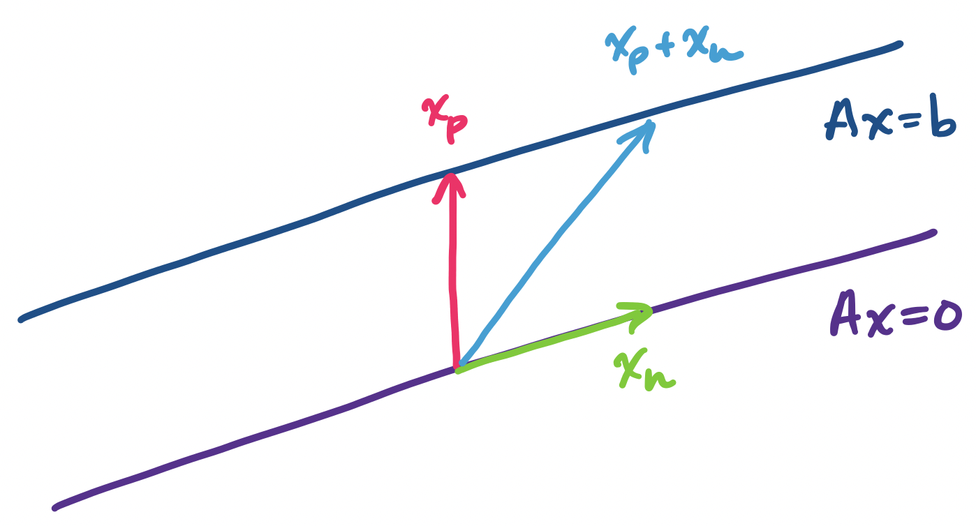
This means that a vector $\mathbf x_n$ will tell us how to move along the null space. But if we add $\mathbf x_p$, this will shift us over to the solution space of $A \mathbf x = \mathbf b$.
Let's go back to the question of solvability. This becomes an issue when we have a row of zeros after performing elimination to acquire a matrix in row-reduced echelon form. How do we get a row of zeros? Some combination of rows must have cancelled them out—in other words, those rows were linearly dependent on the others. So this happens when the number of independent rows in our matrix is strictly less than the total number of rows.
Recall that the number of independent rows (or columns) is the rank of the matrix. This value plays an important role, along with the size of the matrix, that determines the solvability of equations that the matrix is involved with. It looks roughly like this.
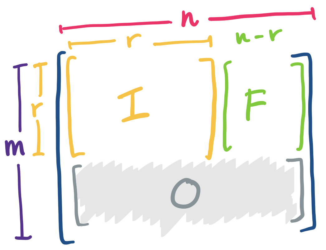
It's clear that the rank is necessarily bounded by the the smaller of $m$ and $n$. This roughly matches our intuition of what happens for matrices of different shapes.
Here is that information in table form.
| $m,n,r$ | Shape of $R$ | Number of solutions |
|---|---|---|
| $r = m = n$ | $\begin{bmatrix} I \end{bmatrix}$ | exactly 1 |
| $r = m \lt n$ | $\begin{bmatrix} I & F \end{bmatrix}$ | infinitely many |
| $m \gt n = r$ | $\begin{bmatrix} I \\ 0 \end{bmatrix}$ | 0 or 1 |
| $r \lt m, n$ | $\begin{bmatrix} I & F \\ 0 & 0 \end{bmatrix}$ | 0 or infinitely many |
The in-between case is where most "real" data will lie. It's unlikely that with very large datasets that we will have full rank in either dimension of the matrix. So this goes back to a question that we briefly mentioned from our earlier example with recommendation systems: what is the $r$ that we need to describe our system. Or conversely, what is the smallest $r$ that we need to approximate our data to a reasonable degree? In this alternative formulation of the question, we realize that it may not be feasible or desirable to try to find the true rank of the matrix.
Another perspective of this idea comes from machine learning. If we think about it, the question of $A \mathbf x = \mathbf b$ can really be thought of as a question about a function $f(x) = b$. In other words, matrices can be thought of like functions. When we're in the in-between case, we have two possibilities:
The original question of machine learning is about "learning" functions in the abstract: Given a set of input-output pairs, we want to approximate a function that satisfies the given pairs. The modern matrix view of this problem is just a specific formulation of the original problem but we can see roughly how it works: we need to provide a subset of data we want our algorithm to "learn" to use for prediction. What's a reasonable subset? One way to figure this out is by thinking about rank.
Here is an extra example dealing with solvability.
Consider the matrix $A = \begin{bmatrix} 3 & 1 \\ 9 & 3 \\ 3 & 4 \\ 2 & 6 \end{bmatrix}$. Suppose we augment it with a column for $\mathbf b$. If we perform elimination on this matrix, we get \[ \begin{bmatrix} 3 & 1 & b_1 \\ 9 & 3 & b_2 \\ 3 & 4 & b_3 \\ 2 & 6 & b_4 \end{bmatrix} \xrightarrow{\substack{(2) - 3 \times (1) \\ (4) - 2 \times (1)}} \begin{bmatrix} 3 & 1 & b_1 \\ 3 & 4 & b_3 \\ 0 & 0 & b_2 - 3b_1 \\ 0 & 0 & b_4 - 2b_1 \end{bmatrix} \xrightarrow{(2) - (1)} \begin{bmatrix} 3 & 1 & b_1 \\ 0 & 3 & b_3 - b_1 \\ 0 & 0 & b_2 - 3b_1 \\ 0 & 0 & b_4 - 2b_1 \end{bmatrix} \\ \xrightarrow{\substack{\frac 1 3 \times (1) \\ \frac 1 3 \times (1)}} \begin{bmatrix} 1 & \frac 1 3 & \frac 1 3 b_1 \\ 0 & 1 & \frac 1 3 (b_3 - b_1) \\ 0 & 0 & b_2 - 3b_1 \\ 0 & 0 & b_4 - 2b_1 \end{bmatrix} \xrightarrow{(1) - \frac 1 2 \times (2)} \begin{bmatrix} 1 & 0 & \frac 4 9 b_1 - \frac 1 9 b_3 \\ 0 & 1 & \frac 1 3 (b_3 - b_1) \\ 0 & 0 & b_2 - 3b_1 \\ 0 & 0 & b_4 - 2b_1 \end{bmatrix} \] We see that with fewer columns than rows, our row-reduced matrix is relatively simple: it's an identity matrix on top of a row of zeros. In this case, we have either one or zero solutions for our system, depending on whether or not the solvability conditions at the bottom of the row-reduced matrix are satisfied. This makes sense: