Matrices as operations
There is one more point to discuss about matrices and matrix products. Let's think back to the view of matrices as functions that transform vectors into other vectors. Just like we did matrix-vector products, we can extend this idea to matrices as functions that transform matrices into other matrices. This leads us to a number of interesting matrices.
The identity matrix $I$ is the matrix such that $AI = A$ and $IA = A$.
Let $A = \begin{bmatrix} 2 & 4 \\ 3 & 4 \end{bmatrix}$ and observe that
\[AI = \begin{bmatrix} A \begin{bmatrix} 1 \\ 0 \end{bmatrix} & A \begin{bmatrix} 0 \\ 1 \end{bmatrix} \end{bmatrix} = \begin{bmatrix} 1 \begin{bmatrix} 2 \\ 3 \end{bmatrix} + 0 \begin{bmatrix} 4 \\ 4 \end{bmatrix} & 0 \begin{bmatrix} 2 \\ 3 \end{bmatrix} + 1 \begin{bmatrix} 4 \\ 4 \end{bmatrix} \end{bmatrix} = \begin{bmatrix} 2 & 4 \\ 3 & 4 \end{bmatrix} = A.\]
In other words, we have a matrix that encodes the linear combination that "selects" the corresponding column in each position. Similarly, we have
\[IA = \begin{bmatrix} I \begin{bmatrix} 2 \\ 3 \end{bmatrix} & I \begin{bmatrix} 4 \\ 4 \end{bmatrix} \end{bmatrix} = \begin{bmatrix} 2 \begin{bmatrix} 1 \\ 0 \end{bmatrix} + 3 \begin{bmatrix} 0 \\ 1 \end{bmatrix} & 4 \begin{bmatrix} 1 \\ 0 \end{bmatrix} + 4 \begin{bmatrix} 0 \\ 1 \end{bmatrix} \end{bmatrix} = \begin{bmatrix} 2 & 4 \\ 3 & 4 \end{bmatrix} = A.\]
The effect of this is the same, but the interpretation can be slightly different.
The identity matrix is a square matrix with ones along its diagonal and zeroes everywhere else. Although we call it the identity matrix, there is really an identity matrix for each size $n$. An interesting question you can work out on your own is: show that there's only one identity matrix of each size $n$.
Generally speaking, this form of a matrix is nice enough to be of note.
A diagonal matrix is a matrix with nonzero entries only along its diagonal and zeroes elsewhere.
Suppose we have a $2 \times 2$ matrix $A = \begin{bmatrix} 2 & 4 \\ 3 & 4 \end{bmatrix}$ and consider the transformation where we simply exchange the columns so we end up with the matrix $B = \begin{bmatrix} 4 & 2 \\ 4 & 3 \end{bmatrix}$. This strange action is also just a bunch of linear combinations put together. Let $\mathbf a_1$ and $\mathbf a_2$ denote the columns of $A$. Then the first column of $B$ is just $0 \cdot \mathbf a_1 + 1 \cdot \mathbf a_2$ and the second column of $B$ is $1 \cdot \mathbf a_1 + 0 \cdot \mathbf a_2$. Putting these two linear combinations together gives us the matrix $\begin{bmatrix} 0 & 1 \\ 1 & 0 \end{bmatrix}$.
We can try the same thing out with three columns. For instance, what if we want to swap columns 1 and 3, while keeping column 2 in place? We reason in the same way: we think about how to construct
- the first column: zero out the other two columns and take the third,
- the second column: zero out the other two columns and take the second,
- the third column: zero out the other two colums and take the third.
From this, we arrive at the matrix $\begin{bmatrix} 0 & 0 & 1 \\ 0 & 1 & 0 \\ 1 & 0 & 0 \end{bmatrix}$.
Linear Equations
The classical problem that linear algebra tries to solve is, given matrix $A$ and vector $\mathbf b$, find all vectors $\mathbf x$ such that
\[A \mathbf x = \mathbf b.\]
This is, of course, the problem of solving a system of linear equations. While the problem itself is not quite so important for our purposes (relatively speaking), thinking about this problem leads to some important insights that we'll make use of.
Suppose we have a system of equations
\begin{align*}
2x + 3y &= 7 \\
4x - 5y &= 11 \\
\end{align*}
We can write this as a matrix $A$ and vectors $\mathbf x$ and $\mathbf b$,
\[\begin{bmatrix} 2 & 3 \\ 4 & -5 \end{bmatrix} \begin{bmatrix}x \\ y \end{bmatrix} = \begin{bmatrix}7 \\ 11 \end{bmatrix}.\]
You probably don't even need linear algebra to solve such problems, given enough time to do it. Perhaps unsurprisingly, thinking about this problem through the lens of linear algebra will give us more insights into the properties of matrices and vectors.
We can think about this problem in two ways. First, in the way that you've probably seen, what we want to do is find real number solutions $x$ and $y$ that satisfy our equations. Secondly, in the way that you're not used to, what we want to do is find a vector $\mathbf x$ that satisfies our equation.
And we can also think about our solutions from another perspective as well. The usual view, as a solution, suggests that we're looking for values that satisfy our constraints—hence solving the equation. But recall that $\mathbf x$ also describes a linear combination of columns of $A$ that produce $\mathbf b$. In this sense, we're looking for descriptions of vectors again.
Typically, we would like one solution (this was likely the running assumption in these kinds of problems you've seen in the past), but that's not the only possibility. We will also be considering the cases where there could also be no solution for this system, or there could be infinitely many solutions. Each of these situations translates into something about our matrix $A$.
- If there's exactly one solution, then we know that the columns of $A$ must be linearly independent. Why? We'll convince ourselves in a bit, but let's move on.
- However, if $A \mathbf x = \mathbf b$ doesn't have any solutions, we can say something about that: there are no linear combinations of columns of $A$ that give us $\mathbf b$!
- But what if there are infinitely many solutions? This suggests that the columns of $A$ are linearly dependent!
The first and last scenarios are linked together, so it's worth asking why and how this must be the case. Suppose $A$ has linearly dependent columns, say $\mathbf u$ and $\mathbf v$. Then I have $\mathbf u = c \mathbf v$ for some scalar $c$. Well, this gives us $\mathbf u - c\mathbf v = \mathbf 0$, which means that there exists a vector $\mathbf y$, which encodes this linear combination such that $A\mathbf y = \mathbf 0$ and $\mathbf y \neq \mathbf 0$. Then I can take another scalar $k$ and get (infinitely) more combinations of these vectors that give me $k A \mathbf y = \mathbf 0$.
Now, notice that $A \mathbf x = A \mathbf x + \mathbf 0 = \mathbf b$. If I have linearly dependent columns, I have infinitely many ways to get $\mathbf 0$. In this case, for some $\mathbf u \neq \mathbf 0$ with $A \mathbf u = \mathbf 0$, I can write $A \mathbf x + \mathbf 0 = A \mathbf x + A \mathbf u = A(\mathbf x + \mathbf u)$, which means $\mathbf x + \mathbf u$ is another solution for $A \mathbf x = \mathbf b$. On the other hand, if I have linearly independent columns, $\mathbf 0$ is the only linear combination of columns of $A$ that gets me $\mathbf 0$.
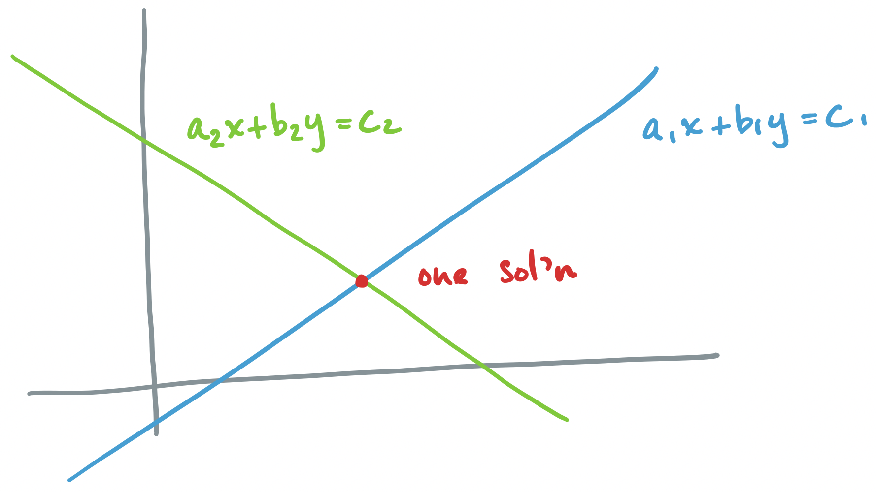
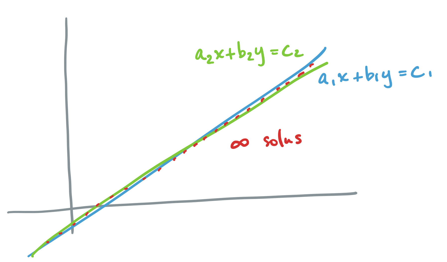
Each of these scenarios can be depicted pictorally, either through the traditional view of geometry (what Strang calls the "row picture"), where equations are drawn as lines or planes on the Euclidean plane, or by the view of linear combinations that we described above (called the "column picture")
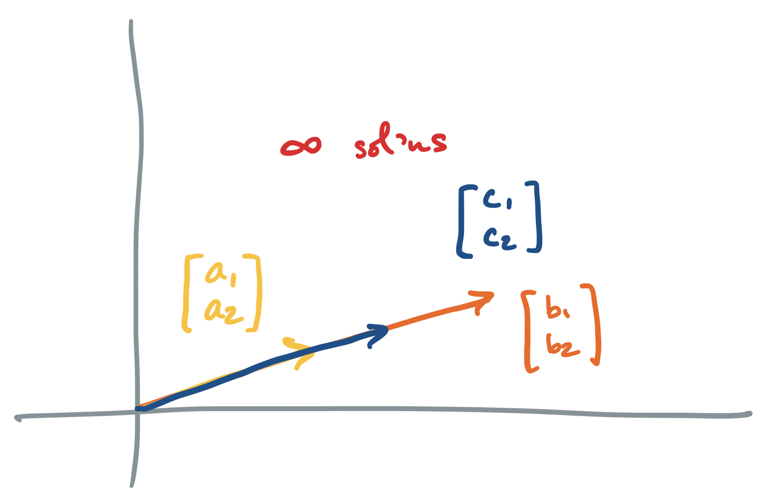
Let's go through each scenario described above, for the system $A \mathbf x = \mathbf b$ where $A = \begin{bmatrix} a_1 & b_1 \\ a_2 & b_2 \end{bmatrix}$ and $\mathbf b = \begin{bmatrix} c_1 \\ c_2 \end{bmatrix}$.
-
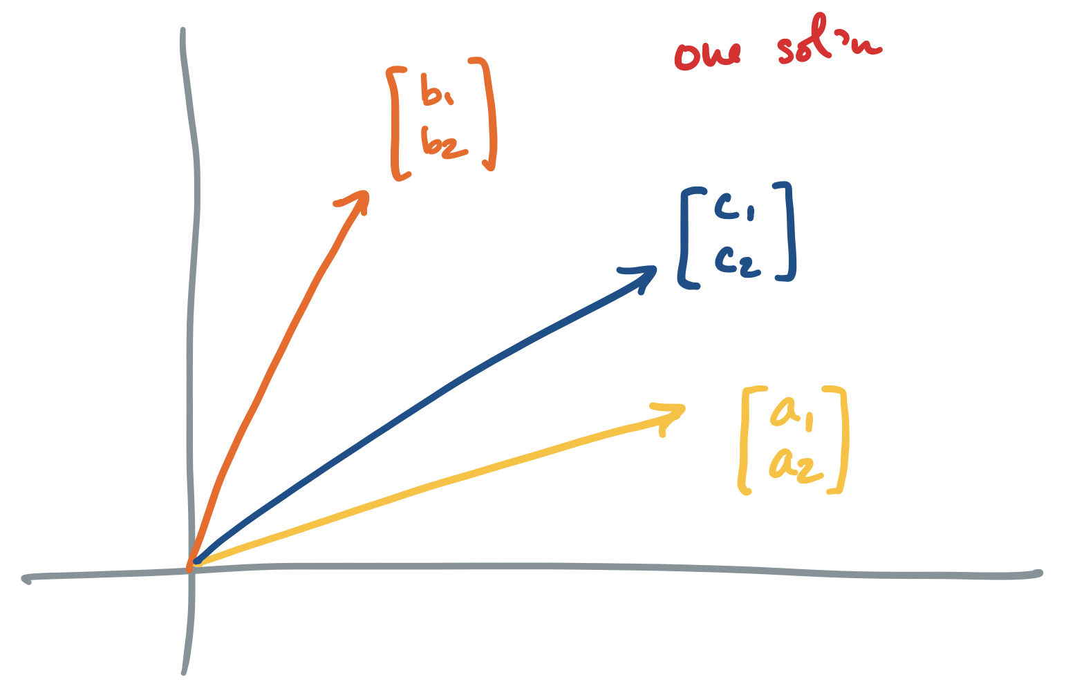
If $A\mathbf x = \mathbf b$ has exactly one solution, the row picture says that there is exactly one point at which all of our equations intersect. The corresponding column picture is that of linearly independent vectors for which there exists one linear combination to describe $\mathbf b$.
-
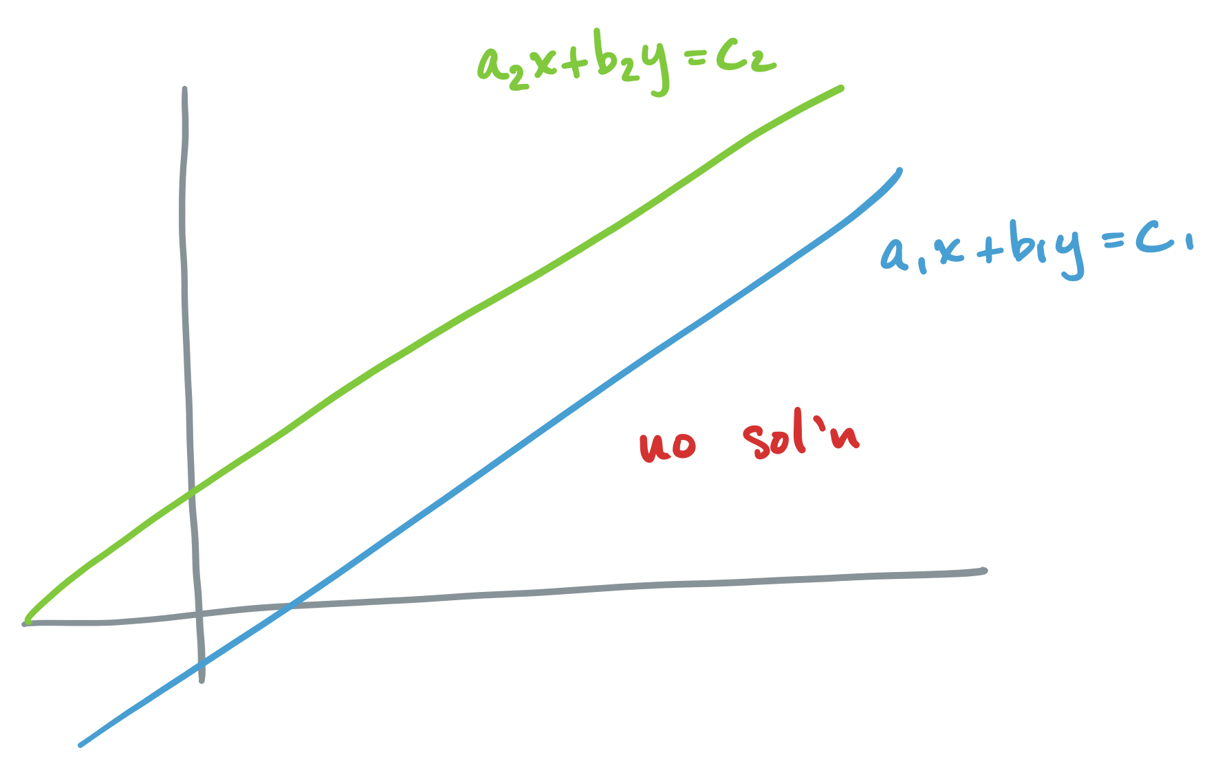
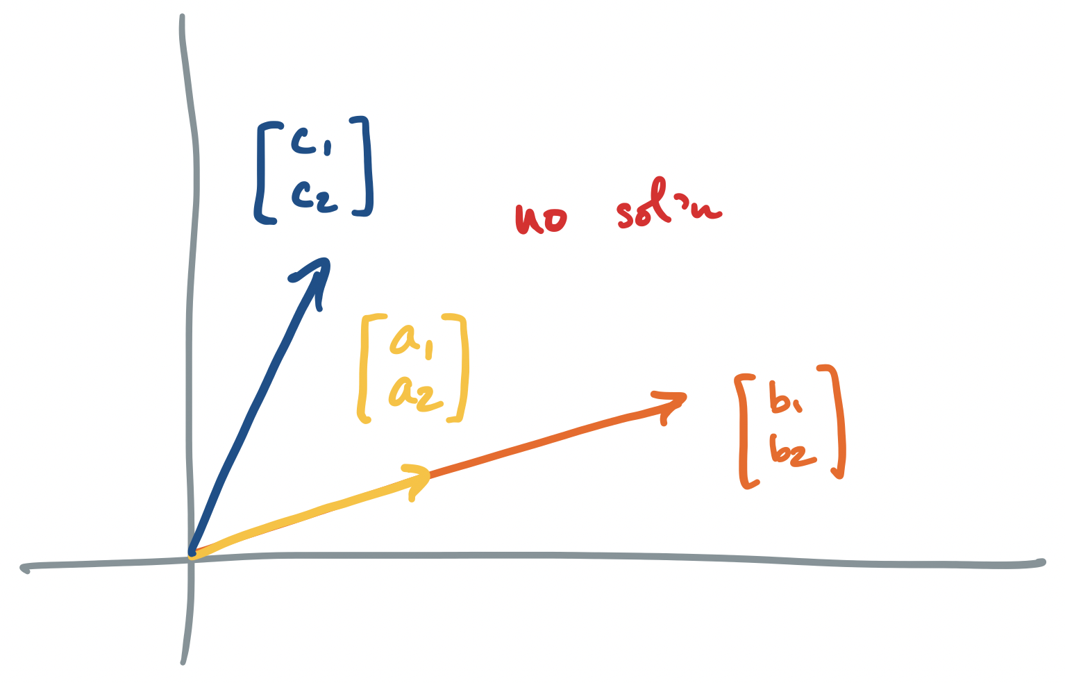
If $A \mathbf x = \mathbf b$ has no solution, we said above that the column picture says that there are no linear combinations of our column vectors that produces $\mathbf b$. The traditional row picture describes two objects (lines, planes, etc) which do not intersect.
-
If $A \mathbf x = \mathbf b$ has infinitely many solutions, we said above that we have linearly dependent columns. So the column picture says that we have infinitely many ways to combine our column vectors to produce $\mathbf b$. The row picture describes two objects (lines, planes, etc) which intersect along at least a line, but maybe even a plane or more in higher dimensions. Since lines are infinitely long, there are infinitely many intersection points.
Dividing by $A$?
Let's dive in and be a bit presumptuous. If we stare at the equation long enough, we realize that what we have is a multiplication problem, and we know how to solve those:
\[\mathbf x = A^{-1} \mathbf b.\]
And so we're done! Of course, there are a few questions that we have to deal with. For example, how does one find the multiplicative inverse of a matrix? But there's a more pressing concern: how do we know that the $A^{-1}$ even exists? This should lead you to interrogate what the meaning of such a matrix should be.
Since $A^{-1}$ itself is a matrix, we can view it in the same way: it's a matrix that describes some collection of vectors. But the above scenarios tell us that it's not always the case that such a matrix always exists. Furthermore, computing such a matrix can be prohibitively expensive. If all we want to do is find $\mathbf x$ for a given $\mathbf b$, then computing $A^{-1}$ can be overkill, if it can be done at all.
It may surprise you that we can't or don't want to find the inverse of a matrix, but we run into this case all the time even just with ordinary numbers. After all, there's no integer that always gives us a half of a number, or more technically, there are no multiplicative inverses of integers that are themselves integers.
Elimination
What we need is a process that will give us $\mathbf x$, if one exists and also tell us whether that's the case. Since we're not interested so much in $A^{-1}$, what we can do is manipulate it in a way that gives us an answer for $\mathbf x$ without necessarily preserving $A$ itself. Why can we do this? It's the same principle as in numerical algebra: apply the same operations to both sides of the equation.
Let's jump ahead to the goal: an upper triangular matrix with non-zero entries on the diagonal. Once we have one of these, computing $\mathbf x$ becomes very easy.
Let $U = \begin{bmatrix} 7 & 6 & 9 \\ 0 & 5 & 6 \\ 0 & 0 & 1 \end{bmatrix}$ such that $U \mathbf x = \begin{bmatrix} -18 \\ -25 \\ -5 \end{bmatrix}$. In other words, we need to solve
\[\begin{bmatrix} 7 & 6 & 9 \\ 0 & 5 & 6 \\ 0 & 0 & 1 \end{bmatrix} \begin{bmatrix} x_1 \\ x_2 \\ x_3 \end{bmatrix} = \begin{bmatrix} -18 \\ -25 \\ -5 \end{bmatrix}.\]
If we turn this into a system of equations, it's not so bad: the final equation gives us something to start with, $x_3 = -5$, and we keep on substituting:
\begin{align*}
5x_2 + 6x_3 & = -25 & 7x_1 + 6x_2 + 9x_3 & = -18 \\
5x_2 + 6 \cdot (-5) &= -25 & 7x_1 + 6 \cdot 1 + 9 \cdot (-5) &= -18\\
5x_2 - 30 &= -25 & 7x_1 - 39 &= -18\\
5x_2 &= 5 & 7x_1 &= 21 \\
x_2 &= 1 & x_1 &= 3
\end{align*}
which gives us $\mathbf x = \begin{bmatrix}3 \\ 1 \\ -5 \end{bmatrix}$.
An $n \times n$ matrix is upper-triangular if its diagonal entries are non-zero and all entries below the diagonal are 0. The diagonal entries are called the pivots.
So the goal is to find a series of operations that we can apply to $A \mathbf x = \mathbf b$ to get $U \mathbf x = \mathbf c$. Again, $\mathbf x$ remains unchanged, because we apply the same transformations to both sides.
What kinds of transformations can we apply? Here, we think back to algebra and solving systems of equations: we want to isolate the final variable so that we can start substituting it into the other equations. We do this by adding multiples of equations to other ones. When viewed as a matrix, this gives us our upper triangular matrix, zeroing out the bottom triangle. This is called elimination.
Consider the matrix $A = \begin{bmatrix} 2 & 1 & 1 \\ 6 & 9 & 8 \\ 4 & -10 & -3 \end{bmatrix}$. We want to transform this into an upper triangular matrix.
First, we need to clear out the entries under the first column. We observe that this can be done by subtracting three of the first row from the second to get
\[\begin{bmatrix} 2 & 1 & 1 \\ 0 & 6 & 5 \\ 4 & -10 & -3 \end{bmatrix}\]
Then we do the same thing with the final row, subtracting two of the first from it.
\[\begin{bmatrix} 2 & 1 & 1 \\ 0 & 6 & 5 \\ 0 & -12 & -5 \end{bmatrix}\]
Now, we need to do the same thing in the second column. We see that we can "subtract" $-2$ of the second row from the third to do this. Note that this is really adding 2 of the second row to the third, but the text likes to refer to all eliminations as subtraction.
\[\begin{bmatrix} 2 & 1 & 1 \\ 0 & 6 & 5 \\ 0 & 0 & 5 \end{bmatrix}\]
And now we have an upper triangular matrix.
How do we encode elimination? Recall that when we eliminate a variable from an equation, we add or subtract some multiple of one equation with the other. In matrices, these are rows, which means what we're really doing is coming up with some linear combination of the rows!
Let's start with columns. Suppose we want to subtract the first column twice from the third column. We start with the identity matrix $I = \begin{bmatrix} 1 & 0 & 0 \\ 0 & 1 & 0 \\ 0 & 0 & 1 \end{bmatrix}$. Now, we know how to describe our combination: $\begin{bmatrix} 1 & 0 & -2 \\ 0 & 1 & 0 \\ 0 & 0 & 1 \end{bmatrix}$. But this isn't what we want—we want to do this with rows! So what do we do if we want to subtract two of the first row from the third? Well, we "flip" or transpose the matrix we came up with: $\begin{bmatrix} 1 & 0 & 0 \\ 0 & 1 & 0 \\ -2 & 0 & 1 \end{bmatrix}$.
Generally speaking, matrices that encode a single elimination step have the same form: 1's along the diagonal, 0's everywhere else, except for the entry representing the elimination step.