CAPP 30271 — Lecture 25

Epilogue: Back to recommender systems

Let's think back to the beginning of the quarter. We had this notion of vectors as objects that could be added together and scaled. These represent objects or data. Since they're finite dimensional, we can focus our attention on $\mathbb R^n$ (things would be a bit different if we considered infinite-dimensional vector spaces).

We are concerned with collections of data, which means we need to work with collections of vectors. Such objects are matrices. Like vectors, we can combine matrices in certain ways, the most significant of which was via matrix multiplication. Matrix multiplication was already enough to lead to our first example: the recommendation system. This was the setup in which our matrix $A$ contained ratings of products by users, with each column representing a user profile and each row representing a product.

At the time, we had the following observations.

• $A = CR$ gives us representative profiles $C$ (i.e. archetypical users) and $R$ combines these profiles to construct each user—the column-centric view of matrix multiplication.
• An alternative view of matrix multiplication says that $A = CR$ gives us representative profiles $R$ (i.e. archetypical products) and $C$ combines these profiles to construct each product—the row-centric view of matrix multiplication.
• The number of columns in $C$ is the rank of $A$ and is typically lower than the number of columns of $A$. This is the same as the number of rows in $R$.

All of this was achieved simply through understanding the mechanism of matrix multiplication. This led to the following questions:

• How do we find $C$ and $R$?
• How do we know which columns should be in $C$?
• How many independent columns do we need in order to get a decent approximation of $A$?
• Realistucally, our matrix would not be complete. How do we interpolate what missing entries of our matrix should be?

These are questions that involve ideas about linear independence, vector spaces, and bases. Over the course of the course, we got some answers.

• Computing the row-reduced echelon form of $A$ will tell us $C$ and $R$.
• This will also tell us the rank of the matrix.

But there's a problem:

• Computing the row-reduced echelon form of $A$ is expensive (especially since $A$ is enormous)!

The singular value decomposition and low-rank approximations close the loop on these questions. SVD combines everything that we've done in the course to give us a way out:

• The SVD gives us a basis for the column space and the row space of $A$—the archetypical profiles.
• The SVD gives us a way to identify which columns/rows are the most important in our matrix, weighted by singular values.
• The SVD gives us an easy way to choose an approximation based on how large we want the rank of our approximation to be.
• Low rank approximations like the one found via SVD can be used for completing matrices.
• There are good algorithms for computing the SVD.

Notice the work required to get here:

• To talk about representative profiles, we needed a notion of vector spaces and basis. To talk about those ideas, we needed the notion of linear combinations, linear indepenence, and linear systems.
• To identify the most important components, we needed to perform spectral analysis.
• To get clean results for each dimension and effective computation of these results, we needed the notion of orthogonality.

These are the basic ingredients for working with matrices and linear data. And these are the basic ideas that machine learning algorithms and data analysis techniques exploit to uncover the latent structures laying hidden inside data. Obviously, there are many more sophsiticated approaches and techniques out there, but they all build on a basic understanding of these fundamental pieces.

Bonus: Lossy compression

We'll lean once more on the idea of the SVD giving us a weighted sum of rank 1 matrices to discuss compression. As mentioned before, the SVD gives us a way to losslessly compress a matrix. By lossless, we mean that the original matrix can be reconstructed perfectly.

However, lossless compression is not viable or necessary in many cases. Much of the digital media we use is compressed lossily: the most widely used image, audio, and video compression algorithms are lossy. The idea behind lossy compression is that exact replication is not necessary because much of the detail that is lost is either undetectable or is just noise.

In some sense, this ties back into the idea of information theory viewed through the lens of machine learning. Machine learning is all about mechanistically trying to find regularities and structure in data. The goal of this is to be able to acquire a simpler description. Such a description is compression in information theoretic terms.

Section 7.2 of the textbook discusses a direct application of this idea: image compression. The idea is that an image is just a grid of pixels. Of course, a matrix is just a grid, so it makes perfect sense to represent an image as a matrix. We can then apply linear algebra tools to process images.

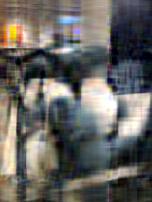
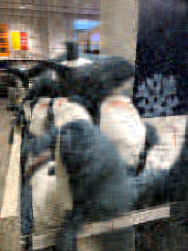
The following images are of the same photo of a pile of Blåhaj at IKEA Shibuya. The original is at the bottom right. From the top left, we have the rank 1, 10, 20, 100, and 200 approximations obtained via SVD (using this convenient online demo).

It's hard to see at the current size on this page, but if you view the images at their actual size, you'll see that there is still a slight but noticeable difference between the rank 100 approximation and the rank 200 approximation, but the rank 200 approximation is virtually indistinguishable from the original.

One can compute approximately how good this compression is based on the sizes of the matrices. The original photo, taken on an iPhone 8, was very large, something like 4000 by 3000-ish pixels (i.e. 12 megapixels). For this exercise, I scaled the original down to 600 by 800 first and used that as the starting point. Such an image results in a matrix of rank 600.

As with any compression method, the effectiveness depends on the amount of regularities in the original image. For instance, images that are flatter and with fewer colours are easier to compress and more complex images will be more difficult to compress.