The idea that we can decompose a matrix for spectral analysis is very exciting, but there's one problem: those matrices must be square (and even then, that's still not enough to guarantee anything!). What about matrices that aren't square (i.e. most of them)? We are not out of luck! We combine everything that we've seen so far to arrive at the following result:
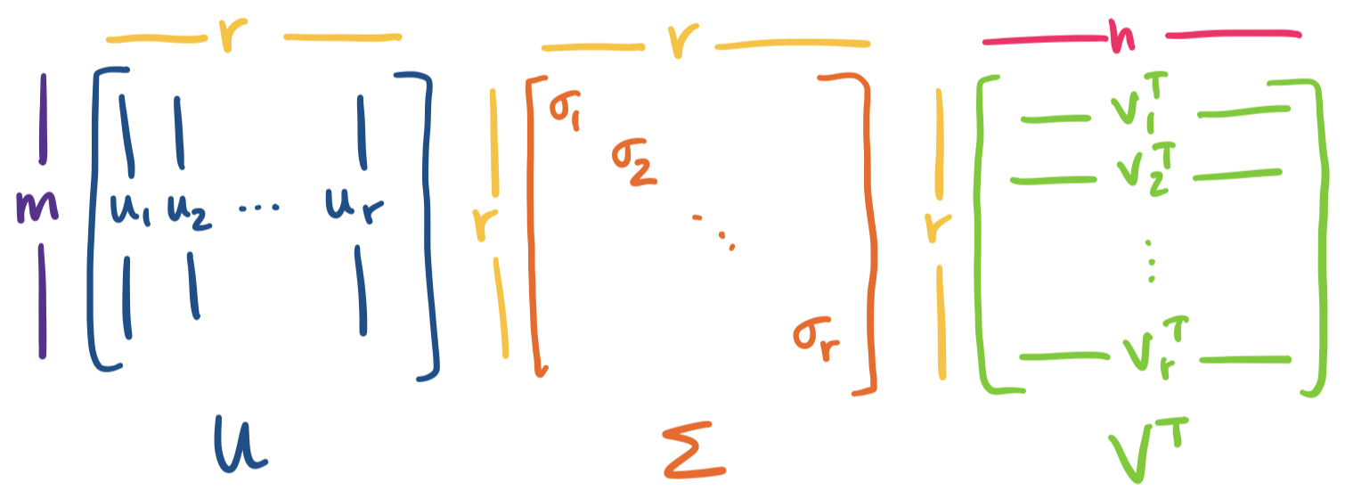
Let $A$ be an $m \times n$ matrix of rank $r$. Then \[A = U \Sigma V^T = \sigma_1 \mathbf u_1 \mathbf v_1^T + \cdots + \sigma_r \mathbf u_r \mathbf v_r^T,\] where $U$ is an orthogonal $m \times r$ matrix, $\Sigma$ is an $r \times r$ diagonal matrix, and $V$ is an orthogonal $n \times r$ matrix.
This factorization of $A$ is called the singular value decomposition of $A$. It's very important to emphasize: the SVD exists for any matrix, no matter its size, shape, invertibility, or anything else.
Let's dissect this.
Visually, we have the following picture:
We get something interesting immediately from this picture. Recall our view of matrix products. Whenever we have $A = BC$, we think of this both as $C$ describing how to combine columns of $B$ to construct columns of $A$ and $B$ describing how to combine rows of $C$ to construct rows of $A$.
We can apply this same interpretation to all matrix decompositions we've seen so far: $A = CR$, $A = LU$, $A = QR$, $A = X \Lambda X^{-1}$. We will apply this view to $A = U \Sigma V^T$ as well.
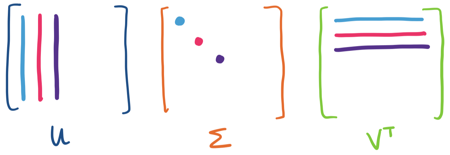
The last few we've seen are a bit puzzling because there are three matrices involved, but we can group them up into two matrices:
However, if we consider the other properties of $U$ and $V$, we can say something ever stronger.
We see that this decomposition is already paying off. Now, we make one further observation: the statement above casts $A$ as a sum of rank 1 matrices defined by the singular vectors of $A$. In particular, each singular value is associated with a specific left and right singular vector. It is this property that we will make use of in order to achieve our main goal: constructing low-rank approximations of $A$.
First, we note an analogy with eigenvalues. If $\mathbf x$ is an eigenvector, then we have $A \mathbf x = \lambda \mathbf x$. The singular values of a matrix give a similar relationship, though it connects two singular vectors, one on the left and one on the right, together rather than a single eigenvector: \[A \mathbf v = \sigma \mathbf u.\]
Let's see that this actually works out.
Consider the matrix $A = \begin{bmatrix} 1 & 2 & 0 \\ 0 & 1 & 2 \end{bmatrix}$. We have two singular vectors $\mathbf v_1 = \begin{bmatrix} 1 \\ 3 \\ 2 \end{bmatrix}$ and $\mathbf v_2 = \begin{bmatrix} -1 \\ -1 \\ 2 \end{bmatrix}$. This gives us \begin{align*} A\mathbf v_1 = \begin{bmatrix} 1& 2 & 0 \\ 0 & 1 & 2 \end{bmatrix} \begin{bmatrix} 1 \\ 3 \\ 2 \end{bmatrix} = \begin{bmatrix} 7 \\ 7 \end{bmatrix} \\ A\mathbf v_2 = \begin{bmatrix} 1& 2 & 0 \\ 0 & 1 & 2 \end{bmatrix} \begin{bmatrix} -1 \\ -1 \\ 2 \end{bmatrix} = \begin{bmatrix} -3 \\ 3 \end{bmatrix} \end{align*} We observe that $\mathbf v_1$ and $\mathbf v_2$ are orthogonal, but not orthonormal. The same holds for the resultant $A \mathbf v_1$ and $A \mathbf v_2$. We can easily normalize them: we see that $\|\mathbf v_1\| = \sqrt 6$ and $\|\mathbf v_2\| = \sqrt{14}$. Normalizing $\mathbf v_1$ and $\mathbf v_2$ would lead us $\mathbf u_1 = \frac 1 {\sqrt 2} \begin{bmatrix} 1 \\ 1 \end{bmatrix}$ and $\mathbf u_2 = \frac 1{\sqrt 2} \begin{bmatrix} -1 \\ 1 \end{bmatrix}$, with singular values $\sigma_1 = \sqrt 7$ and $\sigma_2 = \sqrt 3$.
Putting this together, we have \[AV = \begin{bmatrix} 1& 2 & 0 \\ 0 & 1 & 2 \end{bmatrix} \begin{bmatrix} \frac 1 {\sqrt{14}} & -\frac 1 {\sqrt 6} \\ \frac 3 {\sqrt{14}} & -\frac 1 {\sqrt 6} \\ \frac 2 {\sqrt{14}} & \frac 2 {\sqrt 6} \end{bmatrix} = \frac 1 {\sqrt 2} \begin{bmatrix} 1 & -1 \\ 1 & 1 \end{bmatrix} \begin{bmatrix} \sqrt 7 & 0 \\ 0 & \sqrt 3 \end{bmatrix} = U \Sigma \] Since $V$ is orthonormal, we can write $A = U \Sigma V^T$ to get \[A = \begin{bmatrix} 1& 2 & 0 \\ 0 & 1 & 2 \end{bmatrix} = \frac 1 {\sqrt 2} \begin{bmatrix} 1 & -1 \\ 1 & 1 \end{bmatrix} \begin{bmatrix} \sqrt 7 & 0 \\ 0 & \sqrt 3 \end{bmatrix} \begin{bmatrix} \frac 1 {\sqrt{14}} & \frac 3 {\sqrt{14}} &\frac 2 {\sqrt{14}} \\ -\frac 1 {\sqrt 6} & -\frac 1 {\sqrt 6} & \frac 2 {\sqrt 6} \end{bmatrix}. \] When written in this way, we can see that we have \[A = \sqrt 7 \begin{bmatrix} \frac 1 {\sqrt 2} \\ \frac 1 {\sqrt 2} \end{bmatrix} \begin{bmatrix} \frac 1 {\sqrt{14}} & \frac 3 {\sqrt{14}} &\frac 2 {\sqrt{14}} \end{bmatrix} + \sqrt 3 \begin{bmatrix} -\frac 1 {\sqrt 2} \\ \frac 1 {\sqrt 2} \end{bmatrix} \begin{bmatrix}-\frac 1 {\sqrt 6} & -\frac 1 {\sqrt 6} & \frac 2 {\sqrt 6} \end{bmatrix}. \] or $A = \sigma_1 \mathbf u_1 \mathbf v_1^T + \sigma_2 \mathbf u_2 \mathbf v_2^T$.
In our exampe, we were given $\mathbf v_1$ and $\mathbf v_2$, but where do they come from in the first place? We want to achieve something like diagonalization, so as with diagonalization, we need to find our input and output vectors. For square matrices, we didn't have to think too hard about this: we could just take the eigenvectors and their inverses. For arbitrary matrices, we have a problem: one set of vectors belongs to $\mathbb R^m$ and the other belongs to $\mathbb R^n$. However, we will use our standard trick when it comes to rectangular matrices.
Recall that $A^TA$ is a symmetric $n \times n$ matrix and $AA^T$ is a symmetric $m \times m$ matrix. By the spectral theorem, both of these admit diagonalizations $Q \Lambda A^T$. Now, suppose we know $A = U \Sigma V^T$. Then
In both cases, we have a diagonal matrix, $\Sigma^2$ surrounded by an orthogonal matrix and its transpose. This tells us that
If we were diagonalizing a symmetric matrix, we could stop here, since it's clear how eigenvalues and eigenvectors are related. However, with SVD, we have a bit more work to do: we have to ensure that the left singular vectors and right singular vectors are associated with the correct singular values.
Recall that we have $AV = U\Sigma$. This means that each right singular vector $\mathbf v_k$ will determine the associated left singular vector by the equation \[A \mathbf v_k = \sigma_k \mathbf u_k.\] Of course, in order to know $\mathbf v_k$, we needed to compute $\lambda_k = \sigma_k^2$, so we already have all the pieces to find $\mathbf u_k = \frac{A \mathbf v_k}{\sigma_k}$. Let's convince ourselves that $\mathbf u_k$ is actually a right singular vector. To do that we need to first show that it's an eigenvector of $AA^T$.
Let $\mathbf u_k = \frac{A \mathbf v_k}{\sigma_k}$. Then $\mathbf u_k$ is an eigenvector of $AA^T$ with eigenvalue $\sigma_k^2$.
We see that \[AA^T \mathbf u_k = AA^T \frac{A \mathbf v_k}{\sigma_k} = A \frac{A^TA \mathbf v_k}{\sigma_k} = A \frac{\sigma_k^2 \mathbf v_k}{\sigma_k} = \sigma_k^2 \mathbf u_k.\]
Then, we want to verify that all of these eigenvectors $\mathbf u_k$ are orthonormal.
Let $\mathbf u_j = \frac{A \mathbf v_j}{\sigma_j}$ and $\mathbf u_k = \frac{A \mathbf v_k}{\sigma_k}$. Then $\mathbf u_j$ and $\mathbf u_k$ are orthonormal.
We have \[\mathbf u_j^T \mathbf u_k = \left(\frac{A \mathbf v_j}{\sigma_j}\right)^T \frac{A \mathbf v_k}{\sigma_k} = \frac{\mathbf v_j^T A^TA\mathbf v_k}{\sigma_j\sigma_k} = \frac{\sigma_k}{\sigma_j} \mathbf v_j^T \mathbf v_k.\] Since we started off with the assumption that the right singular vectors are orthonormal, we have that $\mathbf v_j^T \mathbf v_k$ is either 0 or 1, depending on whether or not $j = k$.
From our earlier example, we have \[A A^T = \begin{bmatrix}5 & 2\\2 & 5\end{bmatrix}, \quad A^T A = \begin{bmatrix}1 & 2 & 0\\2 & 5 & 2\\0 & 2 & 4\end{bmatrix}\] The characteristic polynomial for $A^T A$ is \[(1-\lambda)((5-\lambda)(4-\lambda) -4) - 2(2(4-\lambda)) = -\lambda^3(\lambda^2-10\lambda + 21).\] We verify that the characteristc polynomial for $AA^T$ is \[(5-\lambda)^2 - 4 = \lambda^2 - 10 \lambda + 21.\] The nonzero roots of these polynomials are 7 and 3. This then gives us the singular values we saw earlier of $\sqrt 7$ and $\sqrt 3$. One can then solve for the eigenvectors of $A^TA$ in the usual way. Our initial example then shows how these eigenvectors (the right singular vectors of $A$) can be used to obtain the left singular vectors of $A$.
In summary, to compute the SVD for a matrix $A$:
By now, you may have noticed something amiss: our initial definition of the SVD involved matrices of an $m \times r$ matrix $U$, an $r \times r$ diagonal matrix $\Sigma$, and an $n \times r$ matrix $V$. However, the outline of our computation suggests that we have an $m \times m$ matrix $U = AA^T$ and an $n \times n$ matrix $V = A^TA$. If this is the case, we are left with an $m \times n$ matrix $\Sigma$ in order to make the product $U \Sigma V^T$ work. What gives?
The definition we gave earlier is really technically the reduced SVD. The reduced SVD can be thought of as the "useful" part of the SVD. Why?
Suppose we have a matrix $A$ with rank $r \lt m,n$. In this case, $A$ has $r$ nonzero singular values. However, we can end up with more singular values: each of which would be 0. Then what goes in the rest of the "real" $\Sigma$? We would take our $r \times r$ matrix and pad it out with 0's until it is $m \times n$.
Notice that because the rest of the diagonal of $\Sigma$ would be 0s anyway, any additional vectors aren't needed to reconstruct $A$. We would have \begin{align*} A &= \sigma_1 \mathbf u_1 \mathbf v_1^T + \cdots + \sigma_r \mathbf u_r \mathbf v_r^T + \sigma_{r+1} \mathbf u_{r+1} \mathbf v_{r+1}^T + \cdots + \sigma_{\min\{m,n\}} \mathbf u_{\min\{m,n\}} \mathbf v_{\min\{m,n\}}^T\\ &= \sigma_1 \mathbf u_1 \mathbf v_1^T + \cdots + \sigma_r \mathbf u_r \mathbf v_r^T + 0 + \cdots + 0 \\ &= \sigma_1 \mathbf u_1 \mathbf v_1^T + \cdots + \sigma_r \mathbf u_r \mathbf v_r^T \end{align*}
This leads to the next question: what exactly are the missing columns of $U$ and $V$? There are some hints:
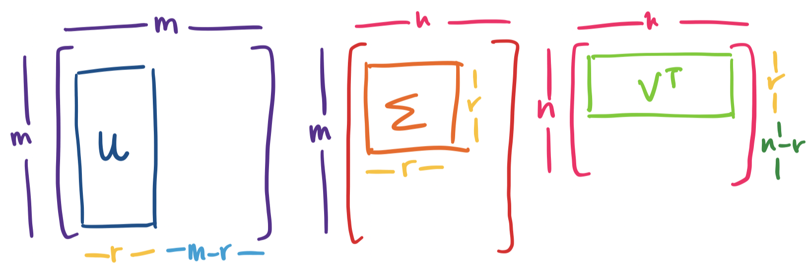
The answer is that the missing columns in $U$ are a basis for the left null space of $A$: they are orthogonal to the first $r$ columns of $U$, which are a basis for the column space of $A$, and there are exactly $m-r$ of them. Similarly, the missing columns in $V$ are a basis for the null space of $A$: they are orthogonal to the first $r$ columns of $V$, a basis for the row space of $A$, and there are exactly $n-r$ of them.
These missing columns together with the matrices we already discussed give us the full singular value decomposition of $A$. In this sense, the SVD really does give us all we want to know about our matrix: not only do we get orthonormal bases for the column and row spaces, like we would expect, but we also get orthonormal bases for the left and ordinary null spaces.
Let $A$ be an $m \times n$ matrix of rank $r$. Then \[A = U \Sigma V^T = \sigma_1 \mathbf u_1 \mathbf v_1^T + \cdots + \sigma_r \mathbf u_r \mathbf v_r^T,\] where $U$ is an orthogonal $m \times m$ matrix, $\Sigma$ is an $m \times n$ diagonal matrix, and $V$ is an orthogonal $n \times n$ matrix such that
If we want to compute the full SVD for $A$, we need to add some steps to our process.
From our example above, we have $A = \begin{bmatrix} 1& 2 & 0 \\ 0 & 1 & 2 \end{bmatrix}$ with the reduced SVD \[U = \frac 1 {\sqrt 2} \begin{bmatrix} 1 & -1 \\ 1 & 1 \end{bmatrix}, \quad \Sigma = \begin{bmatrix} \sqrt 7 & 0 \\ 0 & \sqrt 3 \end{bmatrix}, \quad V = \begin{bmatrix} \frac 1 {\sqrt{14}} & -\frac 1 {\sqrt 6} \\ \frac 3 {\sqrt{14}} & -\frac 1 {\sqrt 6} \\ \frac 2 {\sqrt{14}} & \frac 2 {\sqrt 6} \end{bmatrix}. \] To get the full SVD for $A$, we need to expand $\Sigma$ and $V$. We do not need to change $U$, since it is already the right size ($2 \times 2$). First, we simply pad $\Sigma$ so that it becomes a $2 \times 3$ matrix. We get \[\Sigma = \begin{bmatrix} \sqrt 7 & 0 & 0 \\ 0 & \sqrt 3 & 0 \end{bmatrix}.\]
Then we need to make $V$ a $3 \times 3$ matrix. To do this, we need to compute the null space of $A$. The rref of $A$ is $\begin{bmatrix} 1 & 0 & -4 \\ 0 & 1 & 2 \end{bmatrix}$, which gives us a special solution of $\begin{bmatrix} 4 \\ -2 \\ 1 \end{bmatrix}$.
Here, we note that this vector is orthogonal to the existing columns of $V$, just as we promised. There are two reasons for this:
So all that is left to do is normalize our vector, giving us \[V = \begin{bmatrix} \frac 1 {\sqrt{14}} & -\frac 1 {\sqrt 6} & \frac 4 {\sqrt{21}} \\ \frac 3 {\sqrt{14}} & -\frac 1 {\sqrt 6} & \frac{-2}{\sqrt{21}} \\ \frac 2 {\sqrt{14}} & \frac 2 {\sqrt 6} & \frac{1}{\sqrt{21}} \end{bmatrix}. \]
The significance of the existence of the SVD is both completely natural and kind of astonishing. It is astonishing because it's actually pretty incredible that such a decomposition that contains evertyhing we want to know about our matrix exists—particularly when all of the decompositions we've seen before require our matrices to have special properties.
And yet, this is a completely natural result. If we believe that matrices have certain structures to them, like the fundamental subspaces, and these structures themselves have properties of their own, then of course there should be a decomposition that exposes these structures.
In a way, the SVD is the natural ending point for the work that we've done in this course:
We have one more trick up our sleeve, which is arguably the most useful piece of the SVD: it gives us a convenient tool to describe large, complex, high-dimensional data—low-rank approximations. This is a fitting conclusion to the theme of the course: decomposing large, complex matrices into simpler, tractable parts that expose the underlying structures.