Since we require that an $n \times n$ matrix has $n$ independent eigenvectors, it's not the case that we can always diagonalize a matrix. This situation is a bit like the LU factorization: only invertible matrices can be decomposed in this way. So instead, we need to focus on certain classes of matrices for which we can guarantee an eigendecomposition.
The class of matrices that we're particularly interested in are the symmetric matrices. Recall that symmetric matrices are those that satisfy $A = A^T$—in other words, they're symmetric along their diagonal. We can say the following about them.
Let $S$ be a real symmetric matrix. Then $S = Q\Lambda Q^T$ for some orthogonal matrix $Q$.
Suppose $S$ has a nonzero eigenvalue and a zero eigenvalue. Then $S \mathbf x = \lambda \mathbf x$ and $S \mathbf y = 0 \mathbf y$. These tell us that
This doesn't seem to help us because the column space and null space are not orthogonal complements. However, $S$ is symmetric—this means its row space is the same as its column space. This is enough to give us that $\mathbf x$ and $\mathbf y$ are orthogonal.
But what if we have another non-zero eigenvalue $\alpha$? We have $S \mathbf y = \alpha \mathbf y$. So consider $S - \alpha I$. This gives us $(S - \alpha I) \mathbf y = \mathbf 0$ and $(S - \alpha I) \mathbf x = (\lambda - \alpha)\mathbf x$. Then $\mathbf y$ is in the null space of $S - \alpha I$ and $\mathbf x$ is in the column space of $S - \alpha I$, which is the row space of $S - \alpha I$. So the two vectors are orthogonal.
There are a few things to note here.
Consider the matrix $A = \begin{bmatrix} 2 & -1 & -1 \\ -1 & 2 & -1 \\ -1 & -1 & 2 \end{bmatrix}$. Its characteristic polynomial is $-\lambda(\lambda-3)^2$, so we have $\lambda = 0, 3$.
For $\lambda = 0$, we have $\begin{bmatrix} 2 & -1 & -1 \\ -1 & 2 & -1 \\ -1 & -1 & 2 \end{bmatrix} \mathbf x = 0$. This has rref $\begin{bmatrix} 1 & 0 & -1 \\ 0 & 1 & -1 \\ 0 & 0 & 0 \end{bmatrix}$, which gives us a special solution of $\begin{bmatrix} 1 \\ 1 \\ 1 \end{bmatrix}$.
For $\lambda = 3$, we have $\begin{bmatrix} -1 & -1 & -1 \\ -1 & -1 & -1 \\ -1 & -1 & -1 \end{bmatrix} \mathbf x = 0$. This matrix has an rref of $\begin{bmatrix} 1 & 1 & 1 \\ 0 & 0 & 0 \\ 0 & 0 & 0 \end{bmatrix}$, which gives us special solutions of $\begin{bmatrix} -1 \\ 1 \\ 0 \end{bmatrix}, \begin{bmatrix} -1 \\ 0 \\ 1 \end{bmatrix}$.
If we put these together, we have $\Lambda = \begin{bmatrix} 3 & 0 & 0 \\ 0 & 3 & 0 \\ 0 & 0 & 0 \end{bmatrix}$ and $X = \begin{bmatrix} -1 & -1 & 1 \\ 1 & 0 & 1 \\ 0 & 1 & 1 \end{bmatrix}$. However, we now need to take the extra step of ensuring our eigenvectors are orthonormal. As alluded to in the proof, we don't need to worry about orthogonalizing against all of the vectors, since those with different eigenvalues are already guaranteed to be orthogonal—any such vectors only need to be normalized.
The trickiness comes in when we have multiple eigenvectors for one eigenvalue. We notice that the special solutions we get from solving for the null space are not generally orthogonal. Luckily, this amounts to finding an orthonormal basis for the null space, which we can easily do by applying Gram–Schmidt.
So we take $\begin{bmatrix} -1 \\ 0 \\ 1 \end{bmatrix}$ and use it to find a vector orthogonal to $\begin{bmatrix}-1 \\ 1 \\ 0 \end{bmatrix}$. We get \[\begin{bmatrix} -1 \\ 0 \\ 1 \end{bmatrix} - \begin{bmatrix} -1 \\ 1 \\ 0 \end{bmatrix} \frac{\begin{bmatrix} -1 & 1 & 0 \end{bmatrix} \begin{bmatrix} -1 \\ 0 \\ 1 \end{bmatrix}}{\begin{bmatrix} -1 & 1 & 0 \end{bmatrix} \begin{bmatrix} -1 \\ 1 \\ 0 \end{bmatrix}} = \begin{bmatrix} -1 \\ 0 \\ 1 \end{bmatrix} - \begin{bmatrix} -1 \\ 1 \\ 0 \end{bmatrix} \frac 1 2 = \begin{bmatrix} -\frac 1 2 \\ -\frac 1 2 \\ 1 \end{bmatrix}. \]
So now that our eigenvectors are orthogonalized, we normalize them to get \[Q = \begin{bmatrix} -\frac 1 {\sqrt 2} & -\frac 1 {\sqrt 6} & \frac 1 {\sqrt 3} \\ \frac 1 {\sqrt 2} & -\frac 1 {\sqrt 6} & \frac 1 {\sqrt 3} \\ 0 & \frac 2{\sqrt 6} & \frac 1 {\sqrt 3} \end{bmatrix}.\]
It may be a bit hard to see how eigenvectors and symmetric matrices are used together, so here are some broader examples to give you a flavour of the kinds of things that eigenvectors and symmetric matrices can represent.
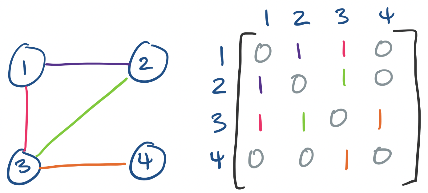
Graphs are a common mathematical structure in discrete mathematics and computer science for representing networks. Graphs of the undirected variety happen to be represented by symmetric matrices.
A graph is a pair of a set $V$ of vertices together with a set of edges which join vertices. Edges are said to be undirected if $(u,v) = (v,u)$.
We can represent graphs as matrices by defining an adjacency matrix: label each vertex from $1$ through $n$. Then entry $a_{ij}$ is 1 if $(i,j)$ is an edge in the graph and 0 otherwise.
We've already made use of this matrix representation when discussing Markov chains. We can get similar results concerning paths like the following:
The number of paths from $u$ to $v$ is $A^k_{u,v}$.
If we have undirected graphs, we must have that $a_{ij} = a_{ji}$. In other words, we have a symmetric matrix. Since we have a symmetric matrix, we know that the adjacency matrix has real eigenvalues and orthonormal eigenvectors. Because of this, the field that studies undirected graphs from the perspective of linear algebra is called spectral graph theory.
The structure of graphs combined with linear algebra leads us to the idea of spectral clustering. This relies on a matrix associated with our graph called the Laplacian.
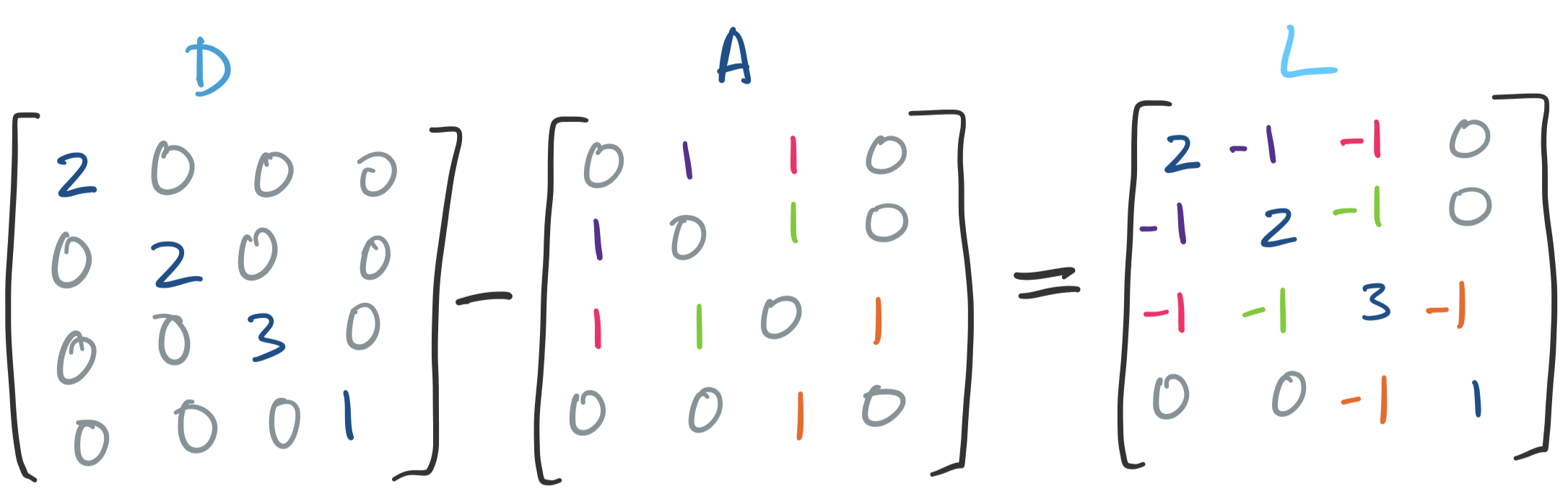
Let $A$ be the adjacency matrix for our graph. We define the degree matrix of our graph by:
\[d_{ij} = \begin{cases} 0& \text{if $i \neq j$}, \\ \deg(i) & \text{if $i = j$.} \end{cases}\]
Recall that the degree of $i$, $\deg(i)$, is the number of edges connected to vertex $i$. So $D$ is a diagonal matrix, where each diagonal entry is the degree of the corresponding vertex. Then we take $L = D - A$. The matrix $L$ is the Laplacian of the graph.
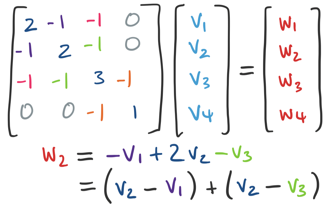
In a sense, the Laplacian tells us how "close" or "far" certain vertices are from each other. Consider a vector $\mathbf v = \begin{bmatrix} v_1 \\ \vdots \\ v_n \end{bmatrix}$ that assigns each vertex $i$ some value $v_i$. We can consider $\mathbf u = L \mathbf v$. What is the $i$th entry of $\mathbf u$? It's the dot product of the $i$th row of $L$ taken with $\mathbf v$:
\[u_i = \deg(i) v_i - \sum_{(i,j) \in E} v_j = \sum_{(i,j) \in E} (v_i - v_j).\]
The eigenvalues and eigenvectors of $L$ encode this information. Consider the expression $\mathbf v^T L \mathbf v$. This is called a quadratic form. Some work expanding the definition will allow you to see that $\mathbf v^T L \mathbf v$ is the sum of all $(v_i - v_j)^2$.
What happens if instead of an arbitrary vector, we use an eigenvector in the quadratic form? For eigenvector $\mathbf u$, we have $\mathbf u^T L \mathbf u = \lambda \mathbf u^T \mathbf u$. If $\mathbf u$ is orthogonal, this tell us that $\sum (u_i-u_j)^2 = \lambda$.
So the nonzero eigenvalues are, roughly speaking, describing how "far" apart certain vertices are: smaller eigenvalues are associated with eigenvectors that keep certain vertices closer together, while larger eigenvalues have vectors that try to maximize that distance between vertices.
The big idea here is that the smallest eigenvalues are associated with eigenvectors that can be thought of as naturally grouping or partitioning certain subsets of vertices together. We can then use these eigenvectors to form clusters.
To cluster, we compute the $k$ smallest eigenvalues and their eigenvectors, $\mathbf u_1, \dots, \mathbf u_k$. Once we have our eigenvectors, we put them together into an $n \times k$ matrix. Each of the $n$ vertices of our graph now corresponds to a row in this matrix and is viewed as a point in $\mathbb R^k$. We then use a $k$-means clustering algorithm to cluster our $n$ points into $k$ clusters.
Why does this work? There is a lot of math involved. The short answer is that the matrix of the graph encodes enough structure that it helps us approximate a computationally hard problem: how to partition a graph into $k$ pieces of roughly equal size. We take advantage of the eigenvectors in two ways:
Where this becomes particularly interesting is when we leave the obvious notions of graph data and focus on similarity. For any set of data, we can compute a similarity graph which is a graph with items as vertices and edges between items are weighted by a similarity score. We can then use this graph as input for a spectral clustering algorithm, which will then cluster our data, which wasn't necessarily graph data in the first place.
A similar idea of using eigenvalues as signals for eigenvectors can be found in PCA. We'll be discussing it in more detail soon, but briefly, the idea and use behind PCA is very similar to linear regression: we are trying to take some high-dimensional data and approximate it with a lower-dimensional subspace. In the case of PCA, we want a set of $k$ orthonormal vectors, the principal components, that describes this subspace.
One key difference between least squares and PCA is that in least squares, the error was defined to be the "vertical" distance of each point from the "line" of best fit (generalizing to higher dimensions as appropriate). In other words, linear regression relies on there being one "special" variable that we're measuring against. PCA generalizes this and looks for "directions", more formally principal components, which ends up being a basis for our low-dimensional subspace approximation. The question is: how do we find these vectors representing the principal components?
This is where thinking about the geometry of eigendecompositions can help. Recall that we can view matrices as transformations. If we can diagonalize $A$, we can separate out these transformations. Consider the transformation $A$ on a vector $\mathbf x$. We know that $A \mathbf x = X \Lambda X^{-1} \mathbf x$. So,
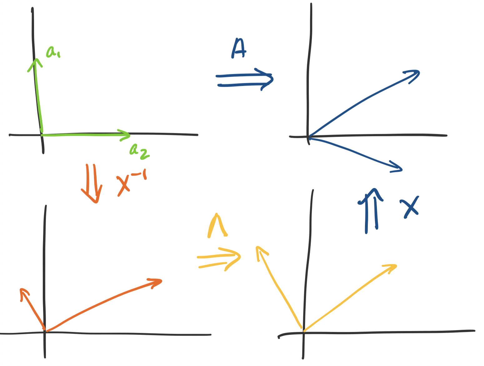
This is not so illuminating because $X$ can really be doing anything, though it's better than nothing—this says that there's a scaling component that $\Lambda$ does, which will be important. But what if we have a symmetric matrix? We know that the diagonalizing matrix is $Q$, an orthogonal matrix.
This lets us nail down the transformation more precisely—$Q$ only "rotates" vectors, since it doesn't change their size at all. How do we know this? The determinant of $Q$ is 1: since $Q^TQ = I$ we have $\det Q \det Q^T = 1$ but $\det Q = \det Q^T$. This tells us that the "space" doesn't change after transformation via $Q$. So we have the following breakdown:
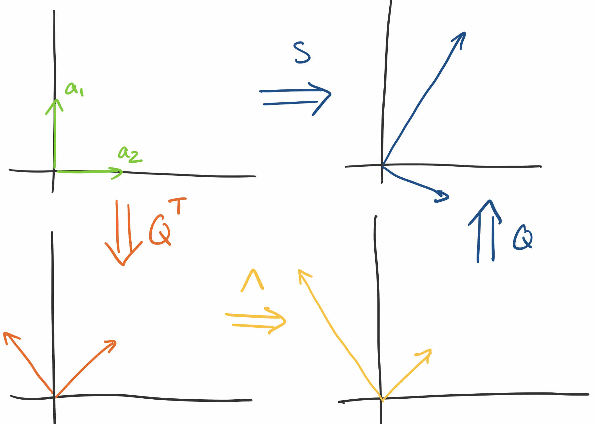
It's clear that all scaling happens in $\Lambda$. This is the key property that PCA relies on: the eigenvector with the largest eigenvalue gives us the direction of most "stretch". So if we want $k$ directions to build our subspace approximation, we simply choose the $k$ eigenvectors associated with the largest eigenvalues.
That's the idea, though we have a bit more to prove why this is the case. Luckily it only involves a bit more geometry and linear algebra to put the idea together.
But notice that this assumes that we can get a symmetric matrix. Luckily, we can get a correlation matrix $A^TA$ from any matrix $A$. This matrix is symmetric, so it must be diagonalizable.
We'll discuss this in more detail when we see that the singular value decomposition leads us back here.