We arrived at the following result last class.
Let $A$ be an $n \times n$ matrix with $n$ linearly independent eigenvectors. Then $AX = X \Lambda$, where $X$ is the matrix of eigenvectors of $A$ and $\Lambda$ is a diagonal matrix of eigenvalues of $A$.
This gives us a definition:
A matrix $A$ is diagonalizable if there exists an invertible matrix $P$ and a diagonal matrix $D$ such that $A = PDP^{-1}$.
So we have that $P = X$, the matrix of eigenvectors, and $D = \Lambda$, the matrix of eigenvalues.
Why is this useful? Remember that a requirement is that $A$ has $n$ linearly independent eigenvectors. This means that the columns of $X$ are all independent—that is, $X$ is invertible. We have the following corollary:
Let $A$ be an $n \times n$ matrix with $n$ linearly independent eigenvectors. Then $A = X \Lambda X^{-1}$ and $\Lambda = X^{-1} A X$.
Consider the matrix $A = \begin{bmatrix} -1 & 0 & -8 \\ 0 & -1 & 8 \\ 0 & 0 & 3 \end{bmatrix}$. Since $A$ is upper triangular, we have that the eigenvalues of $A$ are $-1$ (with multiplicity 2) and $3$.
First, we solve for $\lambda = 3$. In this case, we have the equation \[\begin{bmatrix} -4 & 0 & -8 \\ 0 & -4 & 8 \\ 0 & 0 & 0 \end{bmatrix} \mathbf x = \mathbf 0.\] The rref of this matrix is $\begin{bmatrix} 1 & 0 & 2 \\ 0 & 1 & -2 \\ 0 & 0 & 0 \end{bmatrix}$, so the special solution gives us $\begin{bmatrix} -2 \\ 2 \\ 1 \end{bmatrix}$, which is our eigenvector for $\lambda = 3$.
Next, we consider $\lambda = -1$. We have the equation \[\begin{bmatrix} 0 & 0 & -8 \\ 0 & 0 & 8 \\ 0 & 0 & 4 \end{bmatrix} \mathbf x = \mathbf 0.\] The rref of this matrix is $\begin{bmatrix} 0 & 0 & 1 \\ 0 & 0 & 0 \\ 0 & 0 & 0 \end{bmatrix}$. This gives us a special solution of $\begin{bmatrix} 1 \\ 0 \\ 0 \end{bmatrix}, \begin{bmatrix} 0 \\ 1 \\ 0 \end{bmatrix}$.
This is good because we now have three linearly independent eigenvectors. We can now construct $X = \begin{bmatrix} 1 & 0 & -2 \\ 0 & 1 & 2 \\ 0 & 0 & 1 \end{bmatrix}$, which goes together with $\Lambda = \begin{bmatrix} -1 & 0 & 0 \\ 0 & -1 & 0 \\ 0 & 0 & 3 \end{bmatrix}$.
First, a pressing question: what order do these go in? Based on our "proof" from above, it actually doesn't matter: we can choose an arbitrary order for $X$ and the result of $AX$ should be $X \Lambda$. So all we need to do is make sure that the correct eigenvalues are paired with the right eigenvectors and stick with that order.
To complete the factorization, we compute $X^{-1} = \begin{bmatrix} 1 & 0 & 2 \\ 0 & 1 & -2 \\ 0 & 0 & 1 \end{bmatrix}$.
In summary, we have \[A = \begin{bmatrix} -1 & 0 & -8 \\ 0 & -1 & 8 \\ 0 & 0 & 3 \end{bmatrix} = \begin{bmatrix} 1 & 0 & -2 \\ 0 & 1 & 2 \\ 0 & 0 & 1 \end{bmatrix} \begin{bmatrix} -1 & 0 & 0 \\ 0 & -1 & 0 \\ 0 & 0 & 3 \end{bmatrix} \begin{bmatrix} 1 & 0 & 2 \\ 0 & 1 & -2 \\ 0 & 0 & 1 \end{bmatrix}.\]
This example shows us that although unique eigenvalues guarantee that we have linearly independent eigenvectors, they are not necessary. Because of this, there are actually two different notions of multiplicity:
These can be different: it may be the case that the geometric multiplicity is less than the algebraic multiplicity. In this case, we do not have enough linearly independent eigenvectors to diagonalize our matrix. However, the geometric multiplicity can only be at most the algebraic multiplicity and no greater.
Consider the matrix $A = \begin{bmatrix} -1 & 4 & -8 \\ 0 & -1 & 4 \\ 0 & 0 & 3 \end{bmatrix}$. This matrix has the same eigenvalues as our example from before. This time we will note that the eigenvalue $\lambda = -1$ has algebraic multiplicity 2, since it appears twice as a root of the characteristic polynomial. We will solve for the eigenvectors for $\lambda = -1$.
We arrive at a matrix $\begin{bmatrix} 0 & 4 & -8 \\ 0 & 0 & 4 \\ 0 & 0 & 4 \end{bmatrix}$. The rref for this matrix is $\begin{bmatrix} 0 & 1 & 0 \\ 0 & 0 & 1 \\ 0 & 0 & 0 \end{bmatrix}$. Notice that there are two pivot columns. This means that the null space of this matrix has only one dimension, and so there is only one eigenvector, $\begin{bmatrix} 1 \\ 0 \\ 0 \end{bmatrix}$. Therefore, the geometric multiplicity of $\lambda = -1$ is 1.
This is important because it tells us that not every matrix is diagonalizable. Now that we've been at this course for a while, you might wonder what is wrong with these matrices, but in fact, there's nothing obvious—for example, notice that our matrix is a perfectly fine upper triangular matrix with linearly independent columns. No, diagonalization just happens to be a property that depends on eigenvectors, which we haven't really worked with much until now.
Let's go back to the original motivation for this problem and see how it's resolved. We have the following result that follows right from our decomposition.
Let $A$ be an $n \times n$ matrix that has diagonalization $A = X \Lambda X^{-1}$. Then $A^k = X \Lambda^k X^{-1}$.
To see this, we expand $A^k$ into $(X \Lambda X^{-1})(X \Lambda X^{-1}) \cdots (X \Lambda X^{-1})$. Notice that in between each factor, we have $X^{-1} X = I$.
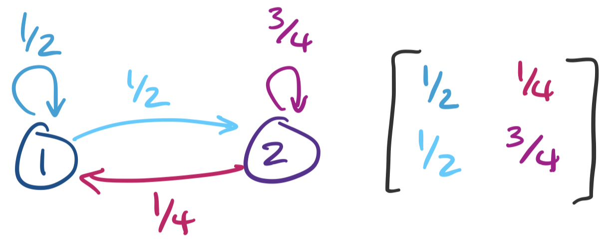
A stochastic matrix, also called a Markov matrix are matrices in which the entries of the matrices are probabilities (i.e. they take on real numbers between 0 and 1) and the sum of the entries of each column is 1.
We can consider one of these matrices $A = \begin{bmatrix} \frac 1 2 & \frac 1 4 \\ \frac 1 2 & \frac 3 4 \end{bmatrix}$. This matrix represents the following Markov chain:
The matrix representation of the Markov chain is the same as any matrix representation for a graph. We label each vertex of our graph 1 through $n$ and label entry $i,j$ by the weight of the edge from vertex $i$ to vertex $j$. Such a matrix is the adjacency matrix for the graph. In this view, a Markov chain is just a weighted directed graph with the property that all outgoing edges of are weighted by probabilities that add up to 1.
Traditionally, the question that we want an answer for is what this system looks like as time goes on. In other words, when we take, say, 100 or 1000 steps on this Markov chain, where do we end up? To answer this, we have to ask what $A^{1000}$ is. To do so, we diagonalize $A$.
First, we see that the characteristic polynomial of $A$ is $\lambda^2 - \frac 5 4 \lambda + \frac 1 4$, which gives us roots $\lambda = 1, \frac 1 4$. This gives us \begin{align*} \lambda &= 1: & \begin{bmatrix} - \frac 1 2 & \frac 1 4 \\ \frac 1 2 & - \frac 1 4 \end{bmatrix} \mathbf x &= \mathbf 0 & \mathbf x &= \begin{bmatrix} \frac 1 2 \\ 1 \end{bmatrix} \\ \lambda & = \frac 1 4: & \begin{bmatrix} \frac 1 4 & \frac 1 4 \\ \frac 1 2 & \frac 1 2 \end{bmatrix} \mathbf x &= \mathbf 0 & \mathbf x &= \begin{bmatrix} -1 \\ 1 \end{bmatrix} \end{align*}
This gives us $X = \begin{bmatrix} 1 & -1 \\ 2 & 1 \end{bmatrix}$ and $\Lambda = \begin{bmatrix} 1 & 0 \\ 0 & \frac 1 4 \end{bmatrix}$. We have that $X^{-1} = \begin{bmatrix} \frac 1 3 & \frac 1 3 \\ - \frac 2 3 & \frac 1 3 \end{bmatrix}$. This gives us \[A^k = \begin{bmatrix} 1 & -1 \\ 2 & 1 \end{bmatrix} \begin{bmatrix} 1 & 0 \\ 0 & \frac 1 4 \end{bmatrix}^k \begin{bmatrix} \frac 1 3 & \frac 1 3 \\ -\frac 2 3 &\frac 1 3 \end{bmatrix}.\]
Again, the question we want to know is what happens when we take many steps. In other words, what happens when $k$ gets very, very large? We take a page from calculus and think about what happens when $k \to \infty$. The effect of $k$ on our diagonal matrix is this: \[A^k = \begin{bmatrix} 1 & -1 \\ 2 & 1 \end{bmatrix} \begin{bmatrix} 1^k & 0 \\ 0 & \left(\frac 1 4\right)^k \end{bmatrix} \begin{bmatrix} \frac 1 3 & \frac 1 3 \\ -\frac 2 3 &\frac 1 3 \end{bmatrix}.\] We recall that $1^k = 1$ no matter how large $k$ gets. However, $\frac 1 {4^k}$ shrinks more and more as $k$ gets larger. As a result, we can treat it as though it becomes 0. So as $k \to \infty$, our system looks more like \[A^k = \begin{bmatrix} 1 & -1 \\ 2 & 1 \end{bmatrix} \begin{bmatrix} 1 & 0 \\ 0 & 0 \end{bmatrix} \begin{bmatrix} \frac 1 3 & \frac 1 3 \\ -\frac 2 3 &\frac 1 3 \end{bmatrix} = \begin{bmatrix} \frac 1 3 & \frac 1 3 \\ \frac 2 3 & \frac 2 3 \end{bmatrix}.\]
This result tells us that as we take more steps in the Markov chain, we have a higher chance of ending up in state 2. This makes sense: while there's an equal probability of going to either state when in state 1, we have a higher chance of staying in state 2 once we've entered it.
The most famous application of this idea is Google's PageRank algorithm, which was described in the late 90s. The idea is that a web "surfer" behaves like a Markov process and the web can be viewed as the Markov chain (really, a directed graph weighted by probabilities). The probability that someone clicks on a link grows depending on both the reputation of where the link is going and where the link is coming from. These reputation scores,represented by an initial vector $\mathbf x$ are then computed by taking $A^k \mathbf x = \mathbf x^*$, where $\mathbf x^*$ is the convergence after large enough $k$.