How do we find eigenvectors? We take our eigenvector equation and rewrite it. The equation $A \mathbf x = \lambda \mathbf x$ becomes \[(A - \lambda I) \mathbf x = \mathbf 0.\] Then this becomes almost the usual question that we've been dealing with all along: solving for $\mathbf x$. Of course, there's an extra step here: what is $\lambda$? To answer that, we have to ask what $A - \lambda I$ is. Obviously, we do not want $A - \lambda I = 0$.
However, if we take a look at this equation, we're back to solving something of the form $B \mathbf x = \mathbf 0$. One vector that satisfies this is $\mathbf x= \mathbf 0$, which we also do we want.
In order for both of these things to be true, it must be the case that $A - \lambda I$ is not invertible—in which case, the null space of $A - \lambda I$ contains more than just the zero vector.
What we need now is a systematic way of computing $\lambda$ based on this information. To do that, we need to discuss the determinant of a matrix.
Determinants are useful quantities that say something important about square matrices (rectangular matrices do not have determinants). Specifically, they quantify the change that a transformation makes to vectors in terms of its "volume". Unfortunately, like matrix inverses, they are a real pain to compute and their properties are not particularly relevant for us. However, we do need them for one thing: being able to compute eigenvalues. This makes sense because both of these values say something about the transformation. So we must discuss how to compute a determinant.
Classically, determinants are defined recursively. We begin with our base case, the $2 \times 2$ matrix.
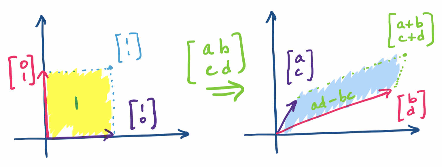
Let $A = \begin{bmatrix} a & b \\ c & d \end{bmatrix}$. Then the determinant of $A$ is $\det A = ad - bc$.
You will sometimes see the determinant denoted by surrounding the matrix with bars instead of square brackets: \[\begin{vmatrix} a & b \\ c & d \end{vmatrix} = ad-bc.\]
What does this say about linear transformations? Consider the effect of this matrix on the standard basis vectors $\begin{bmatrix} 1 \\ 0 \end{bmatrix}$ and $\begin{bmatrix} 0 \\ 1 \end{bmatrix}$.
Notice that this essentially maps every vector onto something like a parallelogram, at least when viewed in $\mathbb R^2$. An interesting question we can ask is what the area of this parallelogram is, viewing the unit box as having an area of 1. This value is exactly the determinant and this is what the determinant signifies—it is the value that quantifies the amount of the transformation.
We can generalize this idea to 3 dimensions (thinking about volume instead of area) or more. The textbook contains details about how the volume arises from this computation in the 3-dimensional case. But we are more concerned with the formula: determinants for a $3 \times 3$ matrix are defined as follows.
Let $A = \begin{bmatrix} a & b & c \\ d & e & f \\ g & h & i \end{bmatrix}$. Then $\det A = a(ei-fh) - b (di-fg) + c(dh-ef)$.
Be careful: notice that the sign for the terms alternates!
The idea here is that we go through each entry in the first row and consider the determinant of the $2 \times 2$ matrix obtained by removing the row and column that the entry is in. That is, \[\det A = a \begin{vmatrix} e & f \\ h & i \end{vmatrix} - b \begin{vmatrix} d & f \\ g & i \end{vmatrix} + c \begin{vmatrix} d & e \\ g & h \end{vmatrix}.\]
For general $n$, we can extend this idea and find that the determinant formula depends on computing the determinant for $n$ different $n-1 \times n-1$ matrices. This definition for the determinant is called the Laplace expansion, due to the 17th c. French mathematician Pierre–Simon Laplace. Notice that because we end up having to compute roughly $n!$ determinants, it is not actually computationally feasible to compute determinants for sufficiently large matrices in this way. For hand computation and small $n$, this will be fine.
Here are some useful properties of determinants.
These properties give us some interesting ideas and in particular lead to faster methods for computing determinants.
Recall that if $A$ is invertible, then it can be decomposed into $A = LU$, where both $L$ and $U$ are triangular matrices. We can make use of these properties: both $\det L$ and $\det U$ can be computed by multiplying their diagonals. Then we have $\det A = \det L \det U$. But what if $A$ isn't invertible? Then $\det A = 0$, which we'll discover when LU factorization fails!
What is the determinant of an orthogonal matrix $Q$? We know that $\det Q = \det Q^T$ and $Q^T Q = I$, so we must have that $\det Q = \pm 1$.
The last property is actually where the definition of singular matrix comes from—we saw this earlier simply as square matrices that are not invertible. If we consider the area/volume view of the determinant, this makes sense: a singular matrix has dependent columns, which means one of the dimensions of our parallelopiped collapses and the resultant space has 0 area/volume.
If you read the text, you'll find that determinants allow you to compute the inverse of a matrix without performing elimination. Personally, I think this is a scam which students are too quick to accept because they're tired of doing elimination. But I find computing the determinant and remembering the process to compute the inverse (called Cramer's rule) even more exhausting than just buckling down and doing the elimination, which we know how to do by now. However, if you're more into memorizing formulas, you may find this a more convenient way to compute the inverse.
Recall that $A - \lambda I$ is not invertible. Then $\det(A - \lambda I) = 0$. This is the key we need to solve for the eigenvalues $\lambda$.
Let $A = \begin{bmatrix} 7 & -9 \\ 2 & -2 \end{bmatrix}$. We have \[A - \lambda I = \begin{bmatrix} 7 - \lambda & -9 \\ 2 & -2-\lambda \end{bmatrix}.\] Then the determinant of this matrix is \[(7-\lambda)(-2-\lambda) -2 \cdot -9 = \lambda^2 - 5\lambda + 4.\] Recall that the determinant is 0, so this suggests that the eigenvalues $\lambda$ are roots of this polynomial. Indeed, we have that this polynomial factors to $(\lambda - 4)(\lambda - 1)$, so we have $\lambda = 4, 1$.
The polynomial $\det(A - \lambda I)$ is the characteristic polynomial of $A$. The eigenvalues of $A$ are the roots of the characteristic polynomial of $A$.
One of the implications from this definition is that an $n \times n$ matrix will have a characteristic polynomial of degree $n$. This comes from having $n$ $\lambda$'s along the diagonal of the matrix $A - \lambda I$.
Once we have our eigenvalues, to find the eigenvectors, we substitute each eigenvalue into $A - \lambda I$ and solve the equation $(A - \lambda I)\mathbf x = \mathbf 0$.
The entire process to find eigenvalues and eigenvectors is summarized:
There are a few things to watch out for at this point.
Finally, here are some useful properties of eigenvalues that, in conjunction with properties of determinants, can help you do some sanity checking on your calculations.
Let $A$ be an $n \times n$ matrix with eigenvalues $\lambda_1, \dots, \lambda_n$.
Suppose $\lambda$ is an eigenvalue of $A$ and $\beta$ is an eigenvalue of $B$. Is $\lambda \beta$ an eigenvalue of $AB$? Consider $AB \mathbf x$, where $\mathbf x$ is an eigenvector. Then $AB \mathbf x = A\beta \mathbf x= \beta \lambda \mathbf x$. This doesn't seem true—it suggests that both $A$ and $B$ share the same eigenvectors to begin with. This leads to an interesting result.
Two $n \times n$ matrices $A$ and $B$ share the same $n$ independent eigenvectors if and only if $AB = BA$.
Recall that matrix multiplication is not generally commutative, so this is a fairly important case.
Eigenvectors present us with another opportunity to decompose a matrix. Suppose first that we happen to have an $n \times n$ matrix $A$ with $n$ independent eigenvectors (not obvious that we can always do this!). We use our usual trick for working with several vectors: make them the columns of a matrix. What do we gain from this?
First, remember that if we have an eigenvector $\mathbf x$, we have that $A \mathbf x \lambda \mathbf x$. Now, suppose we take each eigenvector $\mathbf x_1, \dots, \mathbf x_n$ and put them in a matrix $X$. What is the matrix product $AX$? If we apply the usual column-centric view of matrix multiplication, we have \[AX= A \begin{bmatrix} \mathbf x_1 & \cdots & \mathbf x_n \end{bmatrix} = \begin{bmatrix} \lambda_1 \mathbf x_1 & \cdots & \lambda_n \mathbf x_n \end{bmatrix}.\] To see why this is the case, recall that the $i$th column of $X$ determines the $i$th column of the product $AX$ and it is equal to $A$ multiplied by that column. In this case, the $i$th column of $X$ is $\mathbf x_i$, so $A \mathbf x_i = \lambda_i \mathbf x_i$.
To get the decomposition we're looking for, we now decompose the right hand side. We have \[\begin{bmatrix} \lambda_1 \mathbf x_1 & \cdots & \lambda_n \mathbf x_n \end{bmatrix} = \begin{bmatrix} \mathbf x_1 & \cdots & \mathbf x_n \end{bmatrix} \begin{bmatrix} \lambda_1 & & \\ & \ddots & \\ & & \lambda_n \end{bmatrix} = X \Lambda.\] This is fairly straightforward: our product is simply the rhs of the eigenvector equation, so we split up the eigenvectors and eigenvalues. We denote the eigenvalue matrix by $\Lambda$, which is the uppercase version of $\lambda$. This gives us the following theorem.
Let $A$ be an $n \times n$ matrix with $n$ linearly independent eigenvectors. Then $AX = X \Lambda$, where $X$ is the matrix of eigenvectors of $A$ and $\Lambda$ is a diagonal matrix of eigenvalues of $A$.