We need to find $\mathbf{\hat x}$ in order to find the projection $\mathbf p = A \mathbf{\hat x}$. We have \[\mathbf{\hat x} = (A^T A)^{-1} A^T \mathbf b.\] One complication with this is that we now have to compute the inverse for this and we haven't done too much of that. Luckily, we've had plenty of practice doing elimination for the row-reduced echelon form. The process is pretty much the same:
In fact, we saw this work out the very first time we performed elimination to produce a rref for a matrix.
Once we have found $\mathbf{\hat x}$, it is not hard to find the projection vector $\mathbf p$: \[\mathbf p = A \mathbf{\hat x} = A(A^T A)^{-1} A^T \mathbf b.\] Of course, this is just what we get via straightforward substitution from our previous result. We make one more observation to get the projection matrix: \[P = A(A^T A)^{-1} A^T.\] Again, this is just the matrix that we multiply by $\mathbf b$ from the previous equation.
If we take a closer look at what we've done, we see that it is essentially the same as what we did for projection on a line: \[\mathbf p = \mathbf a \mathbf{\hat x} = \mathbf a \frac{\mathbf a^T \mathbf b}{\mathbf a^T \mathbf a} = \mathbf a (\mathbf a ^T \mathbf a )^{-1} \mathbf a ^T \mathbf b.\]
Suppose we want to project $\mathbf b = \begin{bmatrix} 3 \\ 1 \\ 5 \end{bmatrix}$ onto the subspace spanned by the vectors $\begin{bmatrix} 0 \\ 1 \\ 2 \end{bmatrix}$ and $\begin{bmatrix} 1 \\ 1 \\ 1 \end{bmatrix}$. First, we put our vectors into a matrix $A = \begin{bmatrix} 1 & 0 \\ 1 & 1 \\ 1 & 2 \end{bmatrix}$. Now, the problem becomes projecting $\mathbf b$ onto the column space of $A$. With $A$, we compute $A^TA$, \[\begin{bmatrix} 1 & 1 & 1 \\ 0 & 1 & 2 \end{bmatrix} \begin{bmatrix} 1 & 0 \\ 1 & 1 \\ 1 & 2 \end{bmatrix} = \begin{bmatrix} 3 & 3 \\ 3 & 5 \end{bmatrix}.\] Then we compute $A^T \mathbf b$, \[\begin{bmatrix} 1 & 1 & 1 \\ 0 & 1 & 2 \end{bmatrix} \begin{bmatrix} 3 \\ 1 \\ 5 \end{bmatrix} = \begin{bmatrix} 9 \\ 11 \end{bmatrix}.\]
To solve for $\mathbf{\hat x}$, we need $(A^T A)^{-1}$. We can do this by elimination. \[\begin{bmatrix} 3 & 3 & 1 & 0 \\ 3 & 5 & 0 & 1 \end{bmatrix} \rightarrow \begin{bmatrix} 3 & 3 & 1 & 0 \\ 0 & 2 & -1 & 1 \end{bmatrix} \rightarrow \begin{bmatrix} 1 & 1 & \frac 1 3 & 0 \\ 0 & 1 & -\frac 1 2 & \frac 1 2 \end{bmatrix} \rightarrow \begin{bmatrix} 1 & 0 & \frac 5 6 & -\frac 1 2 \\ 0 & 1 & -\frac 1 2 & \frac 1 2 \end{bmatrix}\] This gives us $(A^TA)^{-1} = \begin{bmatrix} \frac 5 6 & -\frac 1 2 \\ -\frac 1 2 & \frac 1 2 \end{bmatrix}$. We then compute $\mathbf{\hat x} = (A^TA)^{-1} A^T \mathbf b$, \[\begin{bmatrix} \frac 5 6 & -\frac 1 2 \\ -\frac 1 2 & \frac 1 2 \end{bmatrix} \begin{bmatrix} 9 \\ 11 \end{bmatrix} = 9 \begin{bmatrix} \frac 5 6 \\ -\frac 1 2 \end{bmatrix} + 11 \begin{bmatrix} -\frac 1 2 \\ \frac 1 2 \end{bmatrix} = \begin{bmatrix} 2 \\ 1 \end{bmatrix}.\]
Alternatively, we could have set up the system of equations for $A^T A \mathbf{\hat x} = A^T \mathbf b$: \[\begin{bmatrix} 3 & 3 \\ 3 & 5 \end{bmatrix} \begin{bmatrix} \hat x_1 \\ \hat x_2 \end{bmatrix} = \begin{bmatrix} 9 \\ 11 \end{bmatrix},\] which gives us the system \begin{align*} 3\hat x_1 + 3 \hat x_2 &= 9 \\ 3\hat x_1 + 5 \hat x_2 &= 11 \end{align*} From this, it's not too hard to see that $\mathbf{\hat x} = \begin{bmatrix} 2 \\ 1 \end{bmatrix}$.
This then gives us the projection $\mathbf p = A \mathbf{\hat x}$, which is \[\begin{bmatrix} 1 & 0 \\ 1 & 1 \\ 1 & 2 \end{bmatrix} \begin{bmatrix} 2 \\ 1 \end{bmatrix} = 2 \begin{bmatrix} 1 \\ 1 \\ 1 \end{bmatrix} + \begin{bmatrix} 0 \\ 1 \\ 2 \end{bmatrix} = \begin{bmatrix} 2 \\ 3 \\ 4 \end{bmatrix}.\]
Finally, the projection matrix is $P = A(A^TA)^{-1} A^T$, which is
Let's return to our original problem: we want to solve $A \mathbf x = \mathbf b$ but $\mathbf b$ is not in the column space of $A$. This means we want to find $\mathbf x$ that gives us the vector in the column space of $A$ that is closest to $\mathbf b$. This vector is $\mathbf p = A \mathbf{\hat x}$, the projection of $\mathbf b$ onto the column space of $A$.
How do we find $\mathbf{\hat x}$? This depends on the error vector $\mathbf e = \mathbf b - A \mathbf{\hat x}$. Since we want $\mathbf b$ and $\mathbf p$ to be as close as possible, we must have that $\mathbf e$ that minimizes $\|\mathbf e\|$, which means it is perpendicular to the column space. But this means $\mathbf e$ is in the left null space of $A$! This gives us \[A^T\mathbf e = A^T (\mathbf b - A \mathbf{\hat x}) = \mathbf 0,\] so $A^T A \mathbf{\hat x} = A^T \mathbf b$.
In summary, suppose we want to compute the projection of a vector onto a subspace.
Projections allow us to unlock a tool that answers the question of what to do when we are faced with a linear equation $A \mathbf x = \mathbf b$ with no solution. Recall that in such cases, we have a vector that lines outside of the column space of $A$. In practical terms, we have a sample that lies outside of our model for our dataset. This is not an uncommon situation so we can't just throw up our hands and give up. So what to do?
Our discussion of projections has already hinted at this: find the closest point that is in the desired subspace. What this means is that for a matrix $A$, if $\mathbf b$ is not in the column space of $A$, we want to find instead a solution for the vector in the column space of $A$ that is closest to $\mathbf b$. We already have an answer for this: it's the projection of $\mathbf b$ onto the column space of $A$!
The key here is something we mentioned offhandedly earlier: that the projection is the vector in the column space of $A$ for which the error is minimized. Here, the error is the vector $\mathbf e = \mathbf b - \mathbf p$ and the length of that error is $\|\mathbf e\|$.
Recall that by definition, we have $\mathbf p = A \mathbf{\hat x}$, so we have $\mathbf e = \mathbf b - A \mathbf{\hat x}$. By this, we have that $\|\mathbf e\| = \|\mathbf b - A \mathbf{\hat x}\|$. To minimize $\|\mathbf e\|$, we need to minimize $\|\mathbf b - A \mathbf{\hat x}\|^2$, which leads us to what you may know as the least squares approximation.
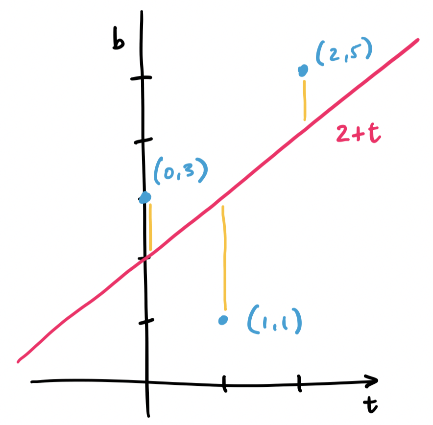
Consider the three points $(0,3), (1,1), (2,5)$. We want to fit a line through these points, but no single line will contain all three. Instead, we find the line that will minimize the distance to all three.
Let's consider a line $y = mx + b$, but call it instead $b = C + Dt$, since many of those variables have been used. What we have with our example is trying to solve the system of equations \begin{align*} C + D \cdot 0 &= 3 \\ C + D \cdot 1 &= 1 \\ C + D \cdot 2 &= 5 \end{align*} This gives us matrices and vectors $A = \begin{bmatrix} 1 & 0 \\ 1 & 1 \\ 1 & 2 \end{bmatrix}$, $\mathbf b = \begin{bmatrix} 3 \\ 1 \\ 5 \end{bmatrix}$, and $\mathbf x = \begin{bmatrix} C \\ D \end{bmatrix}$.
Again, we realize that $\mathbf b$ lies outside of the column space of $A$. This means that there is no solution $C$ and $D$ for our line. So we must instead find $C$ and $D$ for the closest vector that is in the column space. This is our projection, and this makes the question of finding an appropriate $\begin{bmatrix} C \\ D \end{bmatrix}$ the same question as finding $\mathbf{\hat x}$.
Since we've already done this exact example, we have that $C = 2$ and $D = 1$. This gives us the line $2 + t$, which looks like it does a pretty good job of getting close to all of our points.
The least squares solution for an equation $A \mathbf x = \mathbf b$ is $\mathbf{\hat x}$. That is, $\|\mathbf b - A\mathbf x\|^2$ is minimized when $\mathbf x = \mathbf{\hat x}$.
Recall that for any vector $\mathbf b$ in $\mathbb R^m$, it can be written as two vectors: one in the column of an $m \times n$ matrix $A$ and the other in the left null space of that same matrix $A$. We have been calling these $\mathbf p$, the projection of $\mathbf b$ in $\mathbf C(A)$, and $\mathbf e$, the error vector, which belongs to $\mathbf N(A^T)$.
We want to justify that this is the right choice, so we have to think about their lengths—the least squares approximation is the one that minimizes $\|A \mathbf x - \mathbf b\|$, the difference between the desired solution and our best approximation. In other words, we need to solve for $\mathbf x$ so that this quantity is minimized in the following equation: \[\|A\mathbf x - \mathbf b\|^2 = \|A \mathbf x - \mathbf p\|^2 + \|\mathbf e\|^2.\] This is the Pythagorean theorem applied to our vectors of interest. But we have an answer for this: we know that $\mathbf p = A \mathbf{\hat x}$, so choosing $\mathbf x = \mathbf{\hat x}$ makes $\|A\mathbf x-\mathbf p\|^2 = 0$. Since $\mathbf e$ is fixed, this is the best we can do, so $\mathbf{\hat x}$ is our least squares solution.
We can generalize this to any number of points.
Let $(t_1, b_1), \dots, (t_m, b_m)$ be a set of $m$ points. The least squares approximation of a line that goes through all $m$ points is the line $b = C + Dt$, where $\begin{bmatrix} C \\ D \end{bmatrix}$ is the least squares solution to the equation \[\begin{bmatrix} m & \sum\limits_{i=1}^m t_i \\ \sum\limits_{i=1}^m t_i & \sum\limits_{i=1}^m t_i^2 \end{bmatrix} \begin{bmatrix} C \\ D \end{bmatrix} = \begin{bmatrix} \sum\limits_{i=1}^m b_i \\ \sum\limits_{i=1}^m t_ib_i \end{bmatrix}.\]
Suppose we want to fit a line to $m$ points $(t_1, b_1), \dots, (t_m, b_m)$. We would like for this line $b = C + Dt$ to satisfy $b_i = C + Dt_i$ for all of our points, but that is very unlikely. We set up our system in the same way. \[\begin{bmatrix} b_1 \\ \vdots \\ b_m \end{bmatrix} = \begin{bmatrix} 1 & t_1 \\ \vdots & \vdots \\ 1 & t_m \end{bmatrix} \begin{bmatrix} C \\ D \end{bmatrix}.\] This is our equation $\mathbf b = A \mathbf x$. This means we need to find $\mathbf{\hat x}$ by solving $A^T A \mathbf{\hat x} = A^T \mathbf b$.
Let's examine each piece. What is $A^T A$? It is the matrix \[\begin{bmatrix} 1 & \cdots & 1 \\ t_1 & \cdots & t_m \end{bmatrix} \begin{bmatrix} 1 & t_1 \\ \vdots & \vdots \\ 1 & t_m \end{bmatrix} = \begin{bmatrix} 1 \cdot 1 + \cdots + 1 \cdot 1 & 1 \cdot t_1 + \cdots + 1 \cdot t_m \\ t_1 \cdot 1 + \cdots + t_m \cdot 1 & t_1 \cdot t_1 + \cdots + t_m \cdot t_m \end{bmatrix} = \begin{bmatrix} m & \sum\limits_{i=1}^m t_i \\ \sum\limits_{i=1}^m t_i & \sum\limits_{i=1}^m t_i^2 \end{bmatrix} \] Then $A^T \mathbf b$ is \[\begin{bmatrix} 1 & \cdots & 1 \\ t_1 & \cdots & t_m \end{bmatrix} \begin{bmatrix} b_1 \\ \vdots \\ b_m \end{bmatrix} = \begin{bmatrix} 1 \cdot b_1 + \cdots + 1 \cdot b_m \\ t_1 \cdot b_1 + \cdots + t_m \cdot b_m \end{bmatrix} = \begin{bmatrix} \sum\limits_{i=1}^m b_i \\ \sum\limits_{i=1}^m t_ib_i \end{bmatrix}.\]
This is a nice shortcut—you can just apply this formula wihtout having to compute $A^TA$ or $A^T \mathbf b$ step by step.
The textbook only goes as far as fitting lines and parabolas in $\mathbb R^2$, but one can take the technique of adding another variable for fitting to a parabola and instead consider fitting a plane. For instance, instead of considering points $b = C + Dt + Et^2$ one would think of this as $b = C + Ds + Et$. Then we end up with a matrix $A$ that has rows of the form $\begin{bmatrix} 1 & s_i & t_i \end{bmatrix}$ and $\mathbf{\hat x} = \begin{bmatrix} C \\ D\\ E \end{bmatrix}$. We can extend this idea to as many dimensions as we like.
Why would we want to fit points to a plane or even some higher-dimensional subspace? Consider the classical motivation for this: we have too many points but still want to describe our data as a line. If we extend that to our current setting, we still have too many points but possibly also far too many dimensions. We can use a least squares approximation to find a lower-dimensional subspace that can approximate this data.
In a way, this is another version of the scenario we discussed when first talking about projection: we want a way to describe a large, high-dimensional set of data in a lower dimension. In the case of visualization, we choose a meaningful subspace to project our data onto. In the case of least squares approximation, we simply want to find a simpler way to describe our data.
From an information theoretic point of view, this is essentially lossy compression. Compression in information theoretic terms is the technique of finding smaller, simpler descriptions of objects (in this case, large amounts of data). For instance, the most obvious way to describe something is to describe it fully: just copy and list the entirety of our data. But this is often too much and too complex. Instead, our data likely has patterns and structure embedded within it. We can exploit these regularities to find smaller, but slightly less accurate descriptions of our data.
This is important because working with large, complex data means that we often have to approximate and interpolate our dataset. For instance, if we wanted to train a model based on our data, we would need a way to gauge its accuracy. The obvious way: testing it against the entire dataset, is not feasible. Instead, we have to come up with approximations, like a lower-dimensional least squares approximation, that can be computationally feasible to test against.