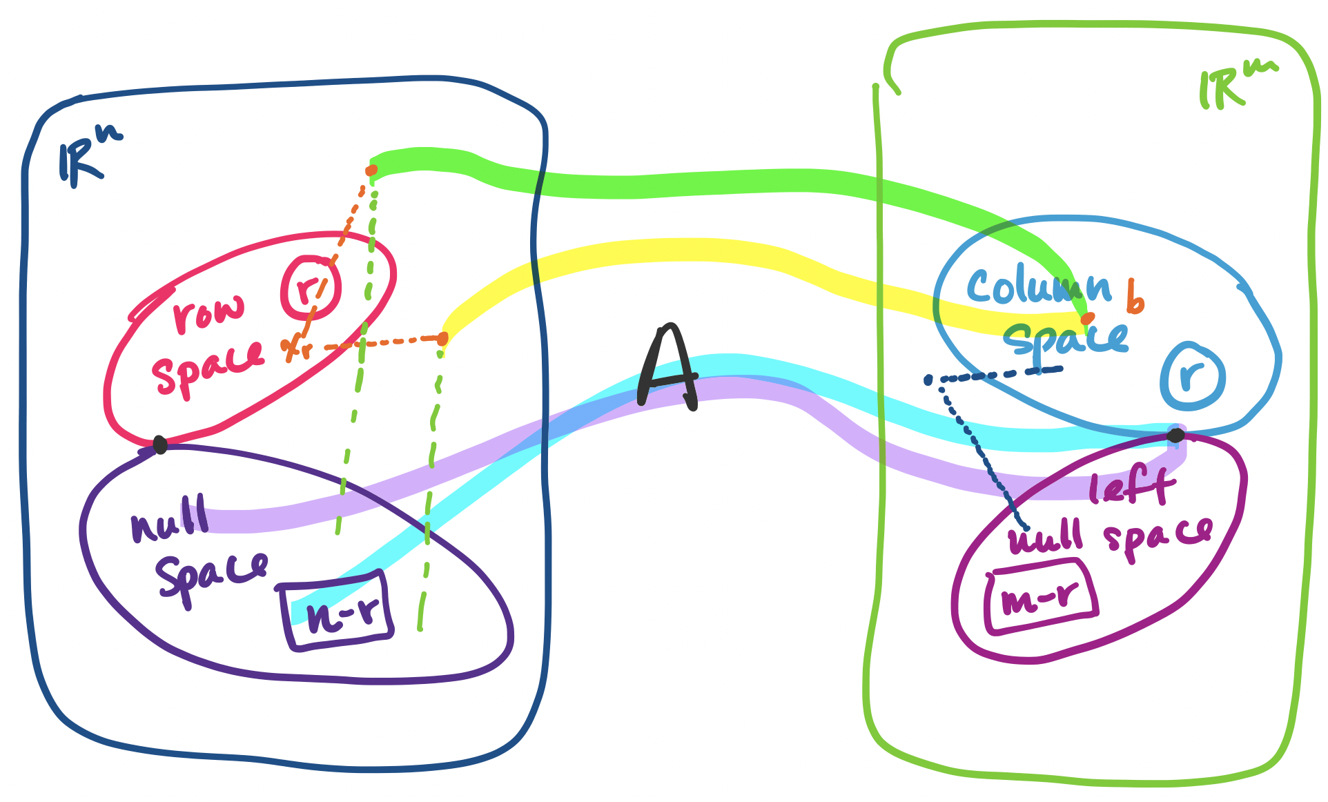
First, a summary. Let $A$ be an $m \times n$ matrix of rank $r$.
| Name | Notation | Subspace of | Dimension |
|---|---|---|---|
| row space | $\mathbf C(A^T)$ | $\mathbb R^n$ | $r$ |
| column space | $\mathbf C(A)$ | $\mathbb R^m$ | $r$ |
| null space | $\mathbf N(A)$ | $\mathbb R^n$ | $n-r$ |
| left null space | $\mathbf N(A^T)$ | $\mathbb R^m$ | $m-r$ |
The left nullspace of an $m \times n$ matrix $A$ is the set of vectors that satisfy $A^T \mathbf y = \mathbf 0$. It is a subspace of $\mathbb R^m$.
Why is this called the left nullspace of $A$? Because we can rewrite the equation $A^T \mathbf y = \mathbf 0$ in terms of $A$ as $\mathbf y^T A = \mathbf 0$. Since $A^T$ is a matrix, it's clear that it has a nullspace, so we can carry out the same proof to find that the left nullspace is a subspace. We will soon see why this subspace is important.
As we've done before, the key to identifying the subspaces is by taking $A$ and transforming it into its row-reduced echelon form $R$. We'll use an example to illustrate this. Let $R = \begin{bmatrix} 1 & 3 & 1 & 0 & 9 \\ 0 & 0 & 0 & 1 & 3 \\ 0 & 0 & 0 & 0 & 0 \end{bmatrix}$. We can see that $R$ is a $3 \times 5$ matrix with rank $r = 2$.
The row space of $R$ has dimension $r$, the rank of $R$. The nonzero rows of $R$ form a basis for the row space of $R$.
In this example, $r = 2$ and there are two nonzero rows. The nonzero rows form a basis for the row space—they are independent since each row has a 1 in the pivot columns and there is no way to combine rows to get those entries.
The column space of $R$ has dimension $r$, the rank of $R$. The pivot columns of $R$ form a basis for the column space of $R$.
In this example $r = 2$ and there are two pivot columns. These pivot columns form a basis for the column space of $R$ (it's pretty clear, since togther, they form $I$).
The null space of $R$ has dimension $n-r$. The special solutions for $R \mathbf x = \mathbf 0$ form a basis for the null space of $R$.
In this example, $R$ has $5-2 = 3$ free variables, so there are three vectors in the special solutions to $R \mathbf x = \mathbf 0$, one for each free variable. They are \[\begin{bmatrix} -3 \\ 1 \\ 0 \\ 0 \\ 0 \end{bmatrix}, \begin{bmatrix} -1 \\ 0 \\ 1 \\ 0 \\ 0 \end{bmatrix}, \begin{bmatrix} -9 \\ 0 \\ 0 \\ -3 \\ 1 \end{bmatrix}.\] We observe that the special solution vectors are independent—there's a 1 in each spot corresponding to the location of the free variable and 0 in the other vectors in the same spot. So the special solutions form a basis for the null space.
The left null space of $R$ has dimension $m-r$.
The left null space of a matrix $A$ is found by finding the special solutions for $A^T$. Since we're dealing $R$, a matrix in rref, solving for its left nullspace is actually quite simple. We first see that we have \[R^T = \begin{bmatrix} 1 & 0 & 0 \\ 3 & 0 & 0 \\ 1 & 0 & 0 \\ 0 & 1 & 0 \\ 9 & 3 & 0 \end{bmatrix}.\] Since we know the rows of $R$ are independent, we can easily tell that the row-reduced echelon form of $R^T$ will be \[\begin{bmatrix} 1 & 0 & 0 \\ 0 & 1 & 0 \\ 0 & 0 & 0 \\0 & 0 & 0 \\0 & 0 & 0 \end{bmatrix}.\] In this case, the null space consists of all vectors $\begin{bmatrix} 0 \\ 0 \\ x_3 \end{bmatrix}$, so an easy basis for it is $\begin{bmatrix} 0 \\ 0 \\ 1 \end{bmatrix}$. This verifies that the dimension of the left null space of $R$ is $3-2=1$.
With this, we have covered all the subspaces for $R$. But the row-reduced echelon form matrix $R$ is shared by many matrices. So we need to take these results and connect them to the respective spaces of $A$.
The row space of $A$ is the row space of $R$.
To see this, we observe that $R$ is computed from $A$ via elimination. But elimnination involves either a permutation of the rows (i.e. a linear combination of the rows of $A$), scaling of rows (i.e. a linear combination of the rows of $A$), or subtracting multiples of one row from another (i.e. a linear combination of the rows of $A$). So because all of our operations are linear combinations of rows from the same row space, we have not changed the row space of the matrix at all.
As a corollary, because the row space of $A$ and $R$ is the same, this means that the dimension of the row space of $A$ and the basis that was computed for the row space of $R$ can be used for the row space of $A$.
The dimension of the column space of $A$ is the dimension of the column space of $R$.
Unfortunately, it is not the case that the column space of $R$ is the same as the column space of $A$—only their dimensions are the same. Consider the following example.
Let $A = \begin{bmatrix} 1 & 3 & 1 & 0 & 9 \\ 0 & 0 & 0 & 1 & 3 \\ 0 & 0 & 0 & 2 & 6 \end{bmatrix}$. Its rref is $R$. However, $\begin{bmatrix} 9 \\ 3 \\ 6 \end{bmatrix}$ is in the column space of $A$, but not in the column space of $R$.
The key difference is that $A$ has nonzero entries in the final row, but $R$ does not. This means the column spaces of the two matrices can't be the same.
So what can we say about the connection between the columns of $A$ and the columns of $R$? Intuitively, when we take combinations of rows of $A$, we are not changing anything about the positions of the columns of $A$ and they interact with each other in the same ways. Recall that we can represent the row elimnination operations as a matrix, say $E$. Then we have \begin{align*} A \mathbf x &= \mathbf 0 \\ EA \mathbf x &= E\mathbf 0 \\ R \mathbf x &= \mathbf 0 \end{align*} This tells us two things: the same combinations of columns in the same positions, specified by $\mathbf x$, gives us $\mathbf 0$. This means that whether a column was independent or not didn't change. This gives us our result: the dimension of the column space of $A$ is the same as that of $R$.
The second thing this tells us that the null space of $A$ and the null space of $R$ are the same.
The null space of $A$ is the null space of $R$.
Technically, there is one more step to take here, since all we've shown is that every vector in the null space of $A$ is in the null space of $R$. To go in reverse, we recall that elimination matrices are invertible, even in their expanded row-reduction form. We take advantage of that to get the following: \begin{align*} R \mathbf x &= \mathbf 0 \\ E^{-1}R \mathbf x &= E^{-1}\mathbf 0 \\ E^{-1}EA \mathbf x &= \mathbf 0 \\ A \mathbf x &= \mathbf 0 \end{align*} Since the null spaces of the two matrices are the same, we get our result that the dimension of the null space of $A$ is $n-r$ for free.
The dimension of the null space space of $A$ is the dimension of the null space space of $R$.
This comes by treating $A^T$ as a matrix and going through our previous arguments. In this case, $A^T$ has $n$ rows and $m$ columns. We know that the dimensions of its row space and column space are $r$. Then we can conclude that its null space must have dimension $m-r$.
Put together, these facts about the dimensions of the fundamental subspaces forms the first part of what the textbook calls the "Fundamental Theorem of Linear Algebra".
Let $A$ be an $m \times n$ matrix of rank $r$.
This is only part 1, which connects the dimensions of the subspaces. This will allow us to work towards a bigger goal: being able to orient these subspaces with each other. We can begin to see something like this when we think about our complete solution.
One of the intriguing suggestions of this result is that a solution to $A \mathbf x = \mathbf b$ can be written as a vector $\mathbf x = \mathbf x_r + \mathbf x_n$—that is, every vector $\mathbf b$ in the column space of $A$ is assocaited with some vector $\mathbf x_r$ in the row space of $A$. (Note: $\mathbf x_r$ is not $\mathbf x_p$, the particular solution) What this tells us that there's an even clearer partitioning of our data than we originally believed.
If $A \mathbf x = \mathbf b$ has a solution, then there is exactly one solution $\mathbf x$ that belongs to the null space.
Again, note that this is not the particular solution. But why does thinking about subspaces help us see this is true? Suppose that there were another vector $\mathbf y$ from the row space such that $A \mathbf y = \mathbf b$. Then we have $A \mathbf x - A \mathbf y = A (\mathbf x - \mathbf y) = \mathbf 0$.
Since we said that both $\mathbf x$ and $\mathbf y$ are in the row space of $A$ and the row space is a subspace, this means that $\mathbf x - \mathbf y$ is also a vector in the row space. But since $A(\mathbf x - \mathbf y) = \mathbf 0$, $\mathbf x - \mathbf y$ is a vector in the null space. But the only vector in both the row space and the null space can only be $\mathbf 0$. So this tells us $\mathbf x = \mathbf y$.
How this $\mathbf x_r$ interacts with vectors $\mathbf x_n$ in the nullspace is something we'll start talking about in the next class. But there's more: this basically says that every vector in $\mathbb R^n$ can be expressed this way. And if this is true, we can say the same for vectors in $\mathbb R^m$: every vector in $\mathbb R^m$ can be written as a vector from the column space of $A$ together with a vector from the left null space of $A$. This is the beginnings of the strategy to being able to say something about how to deal with the question of $A \mathbf x = \mathbf b$ when there is no solution.