Now, we complete the characterization by showing the other direction: that the language of any DFA is regular. We will do this by showing that we can take any DFA and construct a regular expression that recognizes the same language.
Theorem 8.1. Let $A$ be a DFA. Then there exists a regular expression $R$ such that $L(R) = L(A)$.
Proof. Let $A = (Q,\Sigma,\delta,q_0,F)$ and without loss of generality, let $Q = \{1,2,\dots,n\}$. For every pair of states $p,q \in Q$ and integer $k \leq n$, we define the language $L_{p,q}^k$ to be the language of words for which there is a path from $p$ to $q$ in $A$ consisting only of states $\leq k$. In other words, if $w$ is in $L_{p,q}^k$, then for every factorization $w = uv$, we have $\delta(p,u) = r$ such that $r \leq k$ and $\delta(r,v) = q$.
We will show that every language $L_{p,q}^k$ can be defined by a regular expression $R_{p.q}^k$. We will show this by induction on $k$. The idea is that we will begin by building regular expressions for paths between states $p$ and $q$ with restrictions on the states that such paths may pass through and inductively build larger expressions from these paths until we acquire an expression that describes all paths through the DFA with no restrictions.
We begin with $k=0$. Since states are numbered $1$ through $n$, we have two cases:
For our inductive step, we consider the language $L_{p,q}^k$ and assume that there exist regular expressions $R_{p,q}^{k-1}$ for languages $L_{p,q}^{k-1}$. Then we have $$L_{p,q}^k = L_{p,q}^{k-1} \cup L_{p,k}^{k-1} (L_{k,k}^{k-1})^* L_{k,q}^{k-1}.$$ This language expresses one of two possibilities for words traveling on paths between $p$ and $q$. First, if $w \in L_{p,q}^{k-1}$, then $w$ does not travel through any state $k$ or greater between $p$ and $q$.
The other term of the union consists of words $w$ which travel through $k$. The language $L_{p,k}^{k-1}$ is the set of words travelling from $p$ to $k$ restricted to states $\leq k-1$ and the language $L_{k,q}^{k-1}$ is the set of words travelling from $k$ to $q$ restricted to states $\leq k-1$. In between these two languages is $L_{k,k}^{k-1}$, which is the set of words travelling from $k$ back to $k$ without going to any state greater than $k-1$.
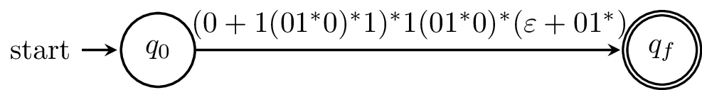
This gives us the regular expression $$R_{p,q}^k = R_{p,q}^{k-1} + R_{p,k}^{k-1} (R_{k,k}^{k-1})^* R_{k,q}^{k-1}.$$ From this, we can conclude that there exists a regular expression $$ R = \sum_{q \in F} R_{q_0,q}^n.$$ Here, $R$ is the regular expression for the language of all words for which there exist a path from $q_0$ to a final state $q \in F$. In other words, $R$ is a regular expression such that $L(R) = L(A)$. $$\tag*{$\Box$}$$
This proof, which is due to McNaughton and Yamada in 1960, gives us an algorithm for computing a regular expression from a DFA. This is nice for computers, but you probably don't want to be executing this by hand, since we have to go through constructing something like $O(n^3)$ different regular expressions. Luckily, for something more human-sized, we can roughly eyeball it.
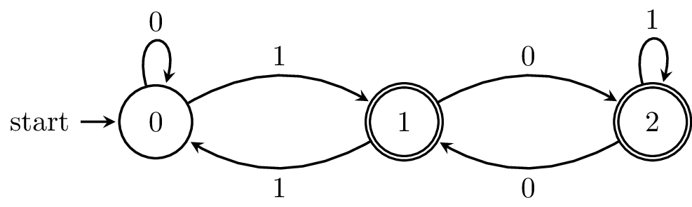
Example 8.2. Consider the following DFA, which is the complement of our "divisible by 3" DFA from two weeks ago. The procedure we're about to carry out is the state-elimination method from Hopcroft, Ullman, and Motwani.
What we'll do is come up with regular expressions by systematically removing states and renaming the labels with regular expressions. Some texts go through the trouble of formally defining these as generalized finite automata, but that's not really necessary because we're just using these as a helpful way to keep track of the regular expressions that we're building and not using them as a real mathematical object.
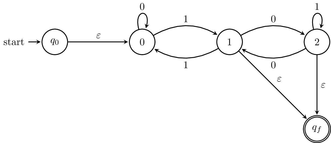
To make things simpler, we begin by adding an initial state and final state and connect $\varepsilon$-transitions as appropriate. Otherwise, we have to contend with the issue of what happens when we try to "eliminate" an initial or final state.
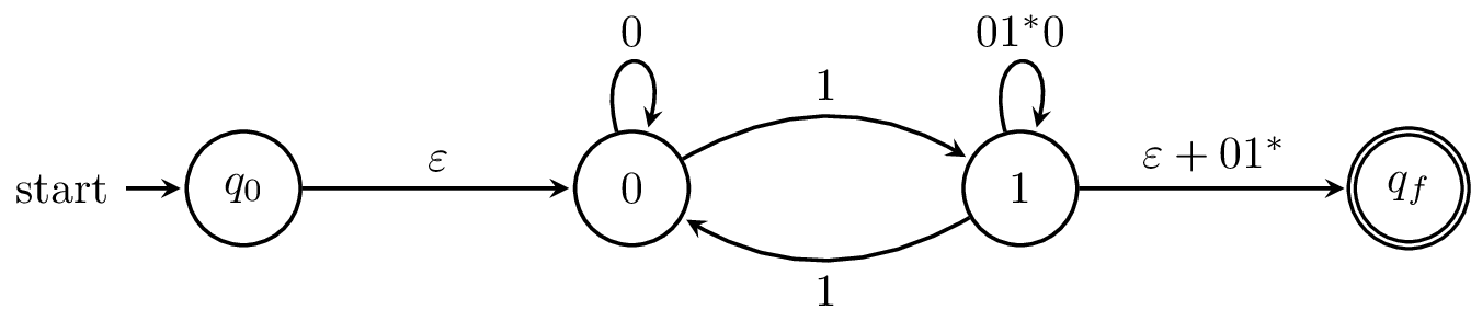
Basically, when we eliminate a state, we replace the transitions to and from the state with regular expressions that represent the strings that would've travelled through it. Consider a path from $1$ through $2$ and back to $1$. This is $1$ followed by any number of $0$s and $1$ again. Similarly, if we didn't go back, we'd be in a final state, so we need to consider that alternative. What this amounts to is figuring out regular expressions for all possible paths through the state we eliminate.
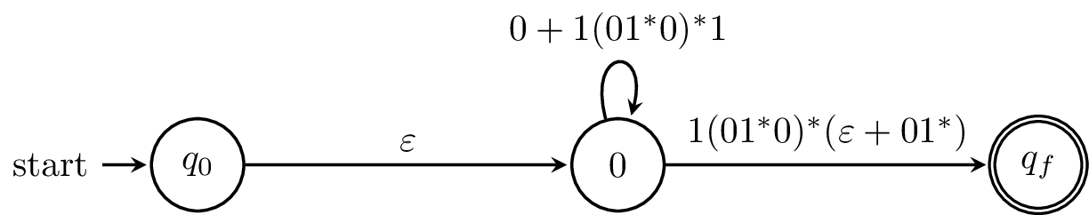
We do this again with all of the states of our original automaton. What we should be left with is a "finite automaton" with a single transition labelled by the regular expression for our language.
In a sense, what we're doing is what the proof of Theorem 8.1 is doing, by constructing regular expressions for part of the machine and combining them. The difference is that we're not doing this for all possible pairs and paths. One consideration of this manual approach is that eliminating states in a different order can produce different regular expressions.
Example 8.3. You may notice that we have sort of the same issue when going from a regular expression to a DFA. The Thompson construction of Theorem 7.7 gives a nice algorithm, but it's not necessarily the most direct way to compute an automaton by hand. Something that may be more satisfying for hand calculation is Glushkov's position automaton.
How this works is that you take a regular expression like $(0+1)^* 0$ and index each symbol by position, like $(0_1 + 1_2)^* 0_3$. Then, including a new start state, you have a state set of $\{0,1,2,3\}$. Transitions between these states are added by determining whether there's a way to get to the "next position" in the regular expression. Below is the automaton for $(0+1)^*0$ that's obtained by this construction.

More formally, given a regular expression $E$, we define $\widetilde E$ to be the indexed expression and $\widetilde{\widetilde E} = E$. We define the sets $\operatorname{pos}(E) = \{1, 2, \dots, |E|\}$ and $\operatorname{pos}_0(E) = \operatorname{pos}(E) \cup \{0\}$ and the functions \begin{align*} \operatorname{first}(E) &= \{i \mid a_i w \in L(\widetilde E)\}, \\ \operatorname{last}(E) &= \{i \mid w a_i \in L(\widetilde E)\}, \\ \operatorname{follow}(E,i) &= \{j \mid u a_i a_j v \in L(\widetilde E)\}. \end{align*} Then $\operatorname{follow}(E,0) = \operatorname{first}(E)$ and $$\operatorname{last}_0(E) = \begin{cases} \operatorname{last}(E) & \text{if $\varepsilon \not\in L(E)$}, \\ \operatorname{last}(E) \cup \{0\} & \text{otherwise}. \end{cases}$$
Then the position automaton for $E$ is $A(E) = (\operatorname{pos}_0(E), \Sigma, \delta_{\mathrm{pos}}, 0, \operatorname{last}_0(E))$, where $$\delta_{\mathrm{pos}}(i,a) = \{j \mid j \in \operatorname{follow}(E,i), a = \widetilde{a_j}\}.$$
Since this construction is based on the symbols in the regular expression, we get an NFA that has about as many states as the length of the regular expression. The tradeoff is that there can be quadratically many transitions. Anne Brüggemann-Klein gave an algorithm for computing the position automaton in time quadratic in the size of the regular expression.
Something else you may notice is that the construction here (and for the Thompson automaton) doesn't necessarily give us the smallest or simplest automaton. We'll revisit this question later on.
Putting Theorems 7.7 and 8.1 together, we get Kleene's theorem, which is the big result of Kleene's 1951 paper that was mentioned earlier. This paper was later published in a journal in 1956.
Something you may notice is that the regular expressions that we've defined are much more simple than the ones we commonly see in many programming languages and other software. Indeed, a lot of regular expression tools have various convenient features. One relevant question we've been asking can be applied here: which language operations can we add to regular expressions without changing their expressive power? Based on some of the results we've already seen, we know that we can enrich our regular expressions with intersection and complement. We can think of other features that appear in Unix regexes, like ranges or character classes and determine whether those give us any additional power or not.
However, some other features, like backtracking, are powerful enough that they can recognize languages which are not regular. What this means is that standard Unix/Posix regular expressions aren't actually regular! A formal study of the power of such "practical" regular expressions was done by Câmpeanu, Salomaa, and Yu in 2003. But what do languages that aren't regular look like? This will be something we'll see next.
Another problem that you can come up with is asking what we can take away and then characterizing what kinds of languages we end up with. The most famous of these is the class of star-free regular languages, which are the class of regular languages that can be defined by regular expressions with concatenation, union, intersection, and complement, but not Kleene star. Marcel-Paul Schützenberger, whose name will come up again later in the course, showed in 1965 that these languages have a connection with aperiodic monoids.
This result is related to a collection of problems on regular expressions called star height problems. In 1963, Lawrence Eggan asked whether every regular language could be expressed using a regular expression without nesting Kleene stars, like $(a_1^* a_2^*)^*$, which would be said to have star-height 2. The tricky thing about these kinds of problems is just because your language can be expressed via an expression with nested stars doesn't mean that you need those stars. For instance, it's clear that $(a^*)^* = a^*$. A less obvious (not the first thing you would think of) example is $\Sigma^* = \overline \emptyset$. It is currently not known whether there exists a regular language with star-height greater than 1.
Now, you might say that since we allow complementation, this is not really fair, so we should go back to the basics with only union, concatenation, and star. Here, we actually get Eggan's original question, which was solved in 1966 by Françoise Dejean and Schützenberger, who proved that there exist regular languages with (restricted) star-height $n$ for every $n \in \mathbb N$. However, this led to another famous problem: coming up with an algorithm for computing the star-height of a language. This was eventually solved 25 years later by Kosaburo Hashiguchi in 1988. This algorithm turns out to be extremely complex, to the point of infeasibility; in 2005, Daniel Kirsten was able to improve the algorithm by bringing it down to $2^{2^{O(n)}}$ worst-case space complexity.
Often, we think of regular languages as being easy and solved and completely understood. However, there are still some old and surprising problems that are a bit more difficult than we tend to associate with regular languages.