We've been talking about Myhill-Nerode equivalence classes, which we can think of as sets of words whose suffixes behave the same way. So if we want to think about what's in the Myhill-Nerode equivalence class for some word $w$, we might want to study the set of words $x$ such that $wx \in L$.
Definition 13.1. The quotient of a language $L$ by a word $w$ is the language $$w^{-1} L = \{x \in \Sigma^* \mid wx \in L\}.$$ Much like how ideas like concatenation, powers, and factors (subwords) invoke analogies to multiplication, the use of the term quotient in this case can be thought of in the same way. The quotient $w^{-1} L$ is what's left when we "factor out" $w$.
As with Myhill-Nerode equivalence classes, we can take quotients on any language. However, a key observation that Brzozowski (same one as the algorithm) made in 1964 was that one can compute a quotient for a regular language via its regular expression. We do this by computing the derivative of a regular expression.
First, we define a "helper" function to indicate whether the language of a given regular expression contains $\varepsilon$.
Definition 13.2. Given a regular expression $R$, we define $\delta$ by $$\delta(R) = \begin{cases} \varepsilon & \text{if $\varepsilon \in L(R)$,} \\ \emptyset & \text{if $\varepsilon \not \in L(R)$.} \end{cases}$$ We can apply this definition to each case of the definition for regular expressions to get
Definition 13.3. Let $R$ be a regular expression. Then the derivative of $R$ with respect to $a \in \Sigma$, $D_a(R)$, is defined recursively by
Theorem 13.4. Let $R$ be a regular expression and let $a \in \Sigma$ be a symbol. Then, $$L(D_a(R)) = a^{-1} L(R) = \{x \in \Sigma^* \mid ax \in L(R)\}.$$
In other words, if $R$ is a regular expression, then $D_a(R)$ is a regular expression representing the language of quotients $a^{-1} L(R)$. We can define an obvious extension to words. Let $w = ax$, where $x \in \Sigma^*$ and $a \in \Sigma^*$. Then $D_w(R) = D_{ax}(R) = D_x(D_a(R))$. This leads to the following very interesting observation.
Theorem 13.5. Let $R$ be a regular expression and let $w \in \Sigma^*$. Then $w \in L(R)$ if and only if $\varepsilon \in L(D_w(R))$.
Proof. We have $$\varepsilon \in L(D_w(R)) \iff \varepsilon \in w^{-1} L(R) \iff w \varepsilon \in L(R) \iff w \in L(R).$$ $\tag*{$\Box$}$
Let's see where this idea takes us.
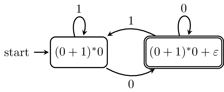
Example 13.6. Let's compute the derivatives for the regular expression $R = (0+1)^* 0$. Let's start with $D_0(R)$. \begin{align*} D_0(R) &= D_0((0+1)^*0) \\ &= D_0((0+1)^*)0 + \delta((0+1)^*)D_0(0) \\ &= D_0((0+1)^*)0 + \varepsilon \varepsilon \\ &= D_0((0+1)^*)0 + \varepsilon \\ &= D_0(0+1)(0+1)^*0 + \varepsilon \\ &= (D_0(0) + D_0(1))(0+1)^*0 + \varepsilon \\ &= (\varepsilon + \emptyset)(0+1)^*0 + \varepsilon \\ &= \varepsilon (0+1)^*0 + \varepsilon \\ &= (0+1)^*0 + \varepsilon \end{align*} Here, the derivative tells us that if we read a $0$, we can either stop ($\varepsilon$) because we skipped the star altogether or go back for another round through the star. Let's call this regular expression $R_1$. First, let's consider $D_1(R)$. \begin{align*} D_1(R) &= D_1((0+1)^*0) \\ &= D_1((0+1)^*)0 + \delta((0+1)^*)D_1(0) \\ &= D_1((0+1)^*)0 + \varepsilon \emptyset \\ &= D_1((0+1)^*)0 \\ &= D_1(0+1)(0+1)^*0 \\ &= (\emptyset + \varepsilon)(0+1)^*0 \\ &= \varepsilon (0+1)^*0 \\ &= (0+1)^*0 \\ &= R \end{align*} This derivative says that if we read a $1$, we can go through another round of the star but we can't stop here. Now let's consider the derivatives on $R_1$. We will see that our job will be slightly easier. \begin{align*} D_0(R_1) &= D_0((0+1)^*0 + \varepsilon) \\ &= D_0((0+1)^*0) + D_0(\varepsilon) \\ &= D_0(R) + \emptyset \\ &= R \end{align*} \begin{align*} D_1(R_1) &= D_1((0+1)^*0 + \varepsilon) \\ &= D_1((0+1)^*0) + D_1(\varepsilon) \\ &= D_1(R) + \emptyset \\ &= R_1 \end{align*}
So we seem to have arrived at two regular expressions that we've seen before. In fact, Brzozowski shows that this is guaranteed to happen.
Theorem 13.7. Every regular expression $R$ has a finite number of distinct derivatives.
This has a few implications. First of all, to compute all the derivatives of a regular expression $R$, we can do what we've done and just keep on computing them until we start getting the same expressions. Obviously, this is not the most efficient way to do this, but we're guaranteed the computation will stop.
But thinking back to the theoretical point of view, recall that these are sets of suffixes of words in our language. And when we consume prefixes of words belonging to these sets, we get different sets, but there are only finitely many of these sets. And finally, we know that those sets that contain $\varepsilon$ correspond to words in the language. This looks suspiciously like the following.
Unlike some of the regular expression to finite automaton constructions we've seen before, this directly gives us a DFA. But there's something even stronger that we can say: the derivatives of a regular expression for a language $L$ correspond to its Myhill-Nerode equivalence classes. In other words, computing the derivatives of a regular expression will give us the minimal DFA for that language. Unfortunately, this method is not what we would consider to be efficient, and the problem of computing a minimal DFA from a regular expression is implied to be quite difficult (PSPACE-complete).
One way around this obstacle is proposed by Antimirov, who defines partial derivatives of a regular expression, which give rise to NFAs rather than DFAs. This method, like the position automaton, produces an NFA of roughly the same size as the length of the regular expression.
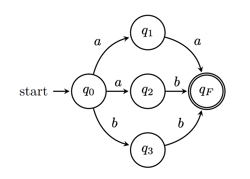
This leads to an interesting question: is there such a thing as a unique minimal NFA? The answer is no. Consider the following NFA.
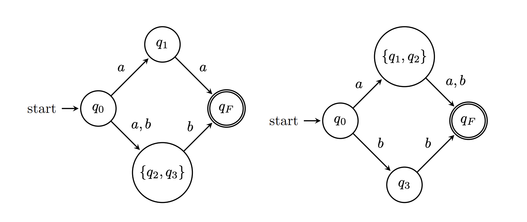
Here are two possible ways to "minimize" this NFA.
Even so, maybe we don't care whether a minimal NFA is unique, we just want to guarantee that we've found a minimal one. Again, we're out of luck. Unlike DFA minimization, NFA minimization is very hard; it's a PSPACE-complete problem. Even trying to restrict our attention to classes of NFAs with very low nondeterminism still only gets us into NP-hardness.
Example 13.8. Let's compute the derivatives for the regular expression $R = (10^*1 + 0)^*$. We have for $0$,
\begin{align*}
D_0(R) &= D_0(10^*1+0) R \\
&= (D_0(10^*1) + D_0(0)) R \\
&= (D_0(10^*1) + \varepsilon) R \\
&= (D_0(1)0^*1 + \delta(1)D_0(0^*1) + \varepsilon) R \\
&= (\emptyset 0^*1 + \emptyset D_0(0^*1) + \varepsilon) R \\
&= \varepsilon R \\
&= R
\end{align*}
So, $D_0(R) = R$, which makes sense: reading $0$ would allows us to start from the beginning of the regular expression since we can just take the star. But for $1$, we have
\begin{align*}
D_1(R) &= D_1(10^*1+0) R \\
&= (D_1(10^*1) + D_1(0)) R \\
&= (D_1(10^*1) + \emptyset) R \\
&= (D_1(1)0^*1 + \delta(1)D_1(0^*1)) R \\
&= (\varepsilon 0^*1 + \emptyset D_1(0^*1)) R \\
&= 0^*1 R \\
&= 0^*1 (10^*1 + 0)^*
\end{align*}
Here, this says that if we read $1$, then we are going to be partially matched to the first term inside the star, and we must finish the rest of the term before going for another round through the star. Let's call this new RE $R_1$ and consider its derivatives. For $0$, we have
\begin{align*}
D_0(R_1) &= D_0(0^*1 R) \\
&= D_0(0^*)1 R + \delta(0^*) D_0(1R) \\
&= D_0(0^*)1 R + \varepsilon D_0(1)R + \delta(1)D_0(R) \\
&= D_0(0^*)1 R + \emptyset R + \emptyset D_0(R) \\
&= D_0(0^*)1 R \\
&= D_0(0) 0^* 1 R \\
&= \varepsilon 0^* 1 R \\
&= 0^* 1 R \\
&= R_1
\end{align*}
Again, we have that reading $0$ doesn't change the regular expression, because we're still in the middle of reading $0$s. Then for $1$, we have
\begin{align*}
D_1(R_1) &= D_1(0^*1 R) \\
&= D_1(0^*)1 R + \delta(0^*) D_1(1R) \\
&= D_1(0^*)1 R + \varepsilon D_1(1)R + \delta(1)D_1(R) \\
&= D_1(0^*)1 R + \varepsilon R + \emptyset D_1(R) \\
&= D_1(0^*)1 R + R \\
&= D_1(0) 0^* 1 R + R \\
&= \emptyset 0^* 1 R + R \\
&= R
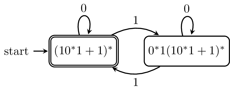
\end{align*}
These derivatives give us the following DFA.
This method lends itself to implementation in functional programming languages. In fact, Stuart Kurtz's CMSC 28000 course notes on derivatives pointed me to a paper detailing the use of derivatives in the regular expression implementations of Standard ML and Scheme (which you probably now know as Racket).
But recall that the notion of a quotient isn't restricted to regular languages. Back in 2010, Matt Might and his co-authors came up with a way to use derivatives on grammars, rather than regular expressions, and to use these derivatives for parsing. Recall that parsing is something that I've said that regular expressions/languages are not capable of. So this sounds very exciting, but this should lead to the following question.
What is a grammar...?
At last, we're ready to step beyond the comfortable world of regular languages and finite automata. Despite having sold this course to you as a course about computation and machines, we're going to be taking a different tack at first and saving the machine model for later. Instead, we'll be looking at grammars.
Like finite automata, context-free grammars were developed in a different context than computation. As you might guess, formal grammars were designed as a way to formally specify grammars for natural language and were developed by Noam Chomsky in 1956. But while the modern treatment of formal grammars was developed relatively recently, the notion of a formal grammar can be traced back to the Indian subcontinent, as far as the 4th century BCE. Here's a simple grammar for a sentence in English: \begin{align*} S & \to NP \enspace VP \\ NP & \to N \mid Art \enspace N \mid Art \enspace Adj \enspace N \\ VP & \to V \mid V \enspace NP \end{align*}
However, despite their origins as a tool to define the grammatical structure of natural language, where they're most commonly found now is in defining the grammatical structure of programming languages. For example, here is the Java Language Specification for Java SE 13. It's in Chapter 19 that we get the good stuff. Here's a snippet, mainly dealing with all of the ways you can write a for statement.
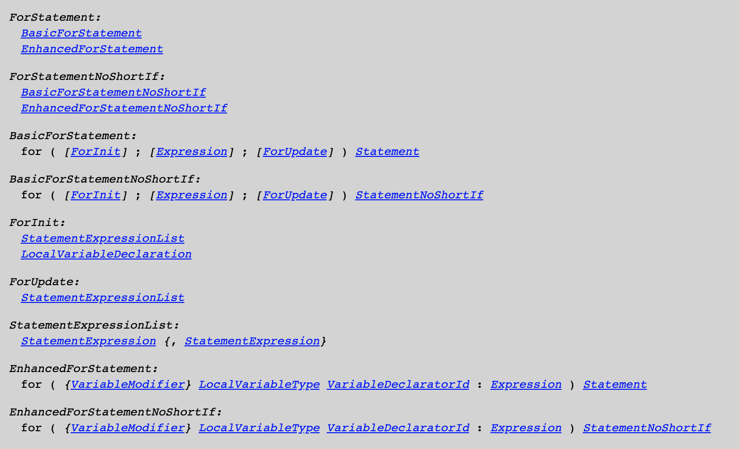
The syntax is not exactly the same, but the idea is.
I mentioned before that in the process of lexical analysis, regular languages are only able to tell us what kinds of tokens it sees, but not whether they're in the correct order. The phase which enforces the correct order of tokens, or whether a string of tokens is "grammatically correct", is called parsing. As you might expect, parsers parse strings and determine their grammatical validity, and as you might guess, parsers are built on context-free grammars.
Now is a good time to have a look at the Chomsky Hierarchy. The hierarchy is due to Chomsky, and categorizes languages by the complexity of their grammars. An important point about the hierarchy is that each class is contained in the more powerful class. This makes sense: every language that can be generated by a right linear grammar can be generated by a more powerful grammar.
| Grammar | Language class | Machine model |
|---|---|---|
| Type-0 (Unrestricted) | Recursively enumerable | Turing machines |
| Type-1 (Context-sensitive) | Context-sensitive | Linear-bounded automata |
| Type-2 (Context-free) | Context-free | Pushdown automata |
| Type-3 (Right/left linear) | Regular | Finite automata |
Interestingly, the hierarchy, although intended for grammars, happens to map very nicely onto automata models.
Definition 14.1. A context-free grammar (CFG) is a 4-tuple $G = (V, \Sigma, P, S)$, where
Usually, it's enough when specifying the grammar to give the set of productions, since any variables and terminals that are used will appear as part of a production.
Let's take a look at an example.
Example 14.2. Let $G = (V,\Sigma,P,S)$, where $V = \{S\}$, $\Sigma = \{a,b\}$, $S$ is the start variable, and $P$ contains the following productions: \begin{align*} S &\to aSb \\ S &\to \varepsilon \end{align*}
It's not too hard to see that the grammar $G$ generates the language $\{a^k b^k \mid k \geq 0\}$. We probably already have an intuitive understanding of how grammars are supposed to generate a language: the idea is that we simply keep on applying as many rules as we like, transforming the word until we end up with a word that contains no variables. Of course, we would like to formalize such a notion.