Recognizable languages are regular
Now, we complete the characterization by showing the other direction: that the language of any DFA is regular. We will do this by showing that we can take any DFA and construct a regular expression that recognizes the same language.
Let $A$ be a DFA. Then there exists a regular expression $\mathbf r$ such that $L(\mathbf r) = L(A)$.
Let $A = (Q,\Sigma,\delta,q_0,F)$ and without loss of generality, let $Q = \{1,2,\dots,n\}$. In other words, we assign each state an integer label from $1$ through $n$.
For each pair of states $p,q \in Q$ and integer $k \leq n$, we define the language $L_{p,q,k}$ to be the language of words for which there is a path from $p$ to $q$ in $A$ consisting only of states with label $\leq k$. In other words, if $w$ is in $L_{p,q,k}$, then for every factorization $w = uv$, we have $\delta(p,u) = r$ such that $r \leq k$ and $\delta(r,v) = q$.
We will show that every language $L_{p,q,k}$ can be described by a regular expression $\mathbf r_{p,q,k}$. We will show this by induction on $k$. The idea is that we will begin by building regular expressions for paths between states $p$ and $q$ with restrictions on the states that such paths may pass through and inductively build larger expressions from these paths until we acquire an expression that describes all paths through the DFA with no restrictions.
We begin with $k=0$. Since states are numbered $1$ through $n$, we have three cases:
- There is no transition from $p$ to $q$, in which case we have $L_{p,q,0} = \emptyset$. Then $\mathbf r_{p,q,0} = \varnothing$.
- There exists $a_1, a_2, \dots, a_m \in \Sigma$ with $\delta(p,a_i) = q$ for $1 \leq i \leq m$ in which case we have $L_{p,q} = \{a_1, a_2, \dots, a_m\}$ for each such transition. Then $\mathbf r_{p,q,0} = \mathtt{a_1 + a_2 + \cdots + a_m}$.
- We have $p = q$, in which case, in addition to the above, we also have $\varepsilon \in L_{p,q,0}$, and we add $\epsilon$ to our regular expression $\mathbf r_{p,q,0}$ as appropriate.
For our inductive step, we consider the language $L_{p,q,k}$ and assume that there exist regular expressions $\mathbf r_{r,s,k-1}$ for languages $L_{r,s,k-1}$ for all states $r,s \in Q$. We claim that we have the following:
$$L_{p,q,k} = L_{p,q,k-1} \cup L_{p,k,k-1} (L_{k,k,k-1})^* L_{k,q,k-1}.$$
This language expresses one of two possibilities for words traveling on paths between $p$ and $q$.
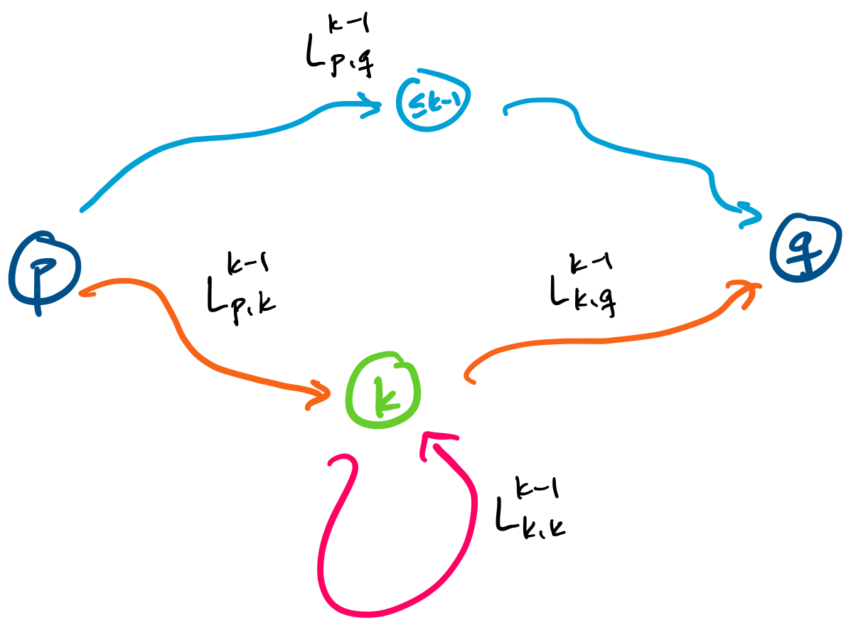
To see this, we first consider when $w \in L_{p,q,k-1}$. In this case, $w$ does not travel through any state $k$ or greater between $p$ and $q$.
The other term of the union consists of words $w$ with $p,q$ paths that contain state $k$. Recall that the language $L_{p,k,k-1}$ is the set of words with paths from $p$ to $k$ restricted to states with label $\leq k-1$ and the language $L_{k,q,k-1}$ is the set of words with paths from $k$ to $q$ restricted to states with label $\leq k-1$. In between these two languages is $L_{k,k,k-1}$, which is the set of words with paths from $k$ back to $k$ without containing any state with label greater than $k-1$.
Since each of the above languages has a regular expression by our inductive hypothesis, we can have the following regular expression:
$$\mathbf r_{p,q,k} = \mathbf r_{p,q,k-1} + \mathbf r_{p,k,k-1} (\mathbf r_{k,k,k-1})^* \mathbf r_{k,q,k-1}.$$
From this, we can conclude that there exists a regular expression
$$ \mathbf r = \sum_{q \in F} \mathbf r_{q_0,q,n}.$$
Here, $\mathbf r$ is the regular expression for the language of all words for which there exist a path from $q_0$ to a final state $q \in F$. In other words, $\mathbf r$ is a regular expression such that $L(\mathbf r) = L(A)$.
This particular proof is due to McNaughton and Yamada in 1960. Notice that we get the recurrence
\[\mathbf r_{p,q,k} = \begin{cases}
\varnothing & \text{if $k = 0$, $p \neq q$, and $\delta(p,a) \neq q$ for all $a \in \Sigma$}, \\
\epsilon & \text{if $k = 0$, $p=q$, and $\delta(p,a) \neq q$ for all $a \in \Sigma$}, \\
\mathtt{a_1 + \cdots + a_n} & \text{if $k = 0$, $p \neq q$, and $\delta(p,a_i) = q$ for $1 \leq i \leq n$}, \\
\mathtt{\epsilon + a_1 + \cdots + a_n} & \text{if $k = 0$, $p = q$, and $\delta(p,a_i) = q$ for $1 \leq i \leq n$}, \\
\mathbf r_{p,q,k-1} + \mathbf r_{p,k,k-1} (\mathbf r_{k,k,k-1})^* \mathbf r_{k,q,k-1} & \text{if $k \gt 0$}, \\
\end{cases}\]
If you’ve studied algorithms before, then you’ll recognize this as a Bellman equation. So this proof gives us a dynamic programming algorithm for computing a regular expression from a DFA.
The trick that’s used here may seem familiar to you if you’ve seen the Floyd-Warshall algorithm for computing all-pairs shortest paths, because it operates on the same idea of progressively constructing paths by constraining the allowed intermediary vertices. (Why are we able to use basically the same algorithm? Because both the shortest paths and DFA to regular expression problems are based on objects that form semirings)
This result, together with the result from last class give us Kleene’s theorem.
Let $\Sigma$ be an alphabet. A language over $\Sigma$ is regular if and only if it is recognized by a finite automaton over $\Sigma$. That is, a language is regular if and only if it is recognizable—$\operatorname{\mathsf{Rec}} \Sigma^* = \operatorname{\mathsf{Reg}} \Sigma^*$.
This result is due to Kleene in 1951, and was later published in 1956.
But let’s think a bit more about the algorithm we just saw. It’s well known that Floyd-Warshall, and by extension the McNaughton and Yamada algorithm, have a running time of $O(n^3)$, which makes sense considering the Bellman equation we saw. However, we probably don’t want to be filling out the dynamic programming table by hand for this. Luckily, we can use what we’ve seen to compute an expression by hand.
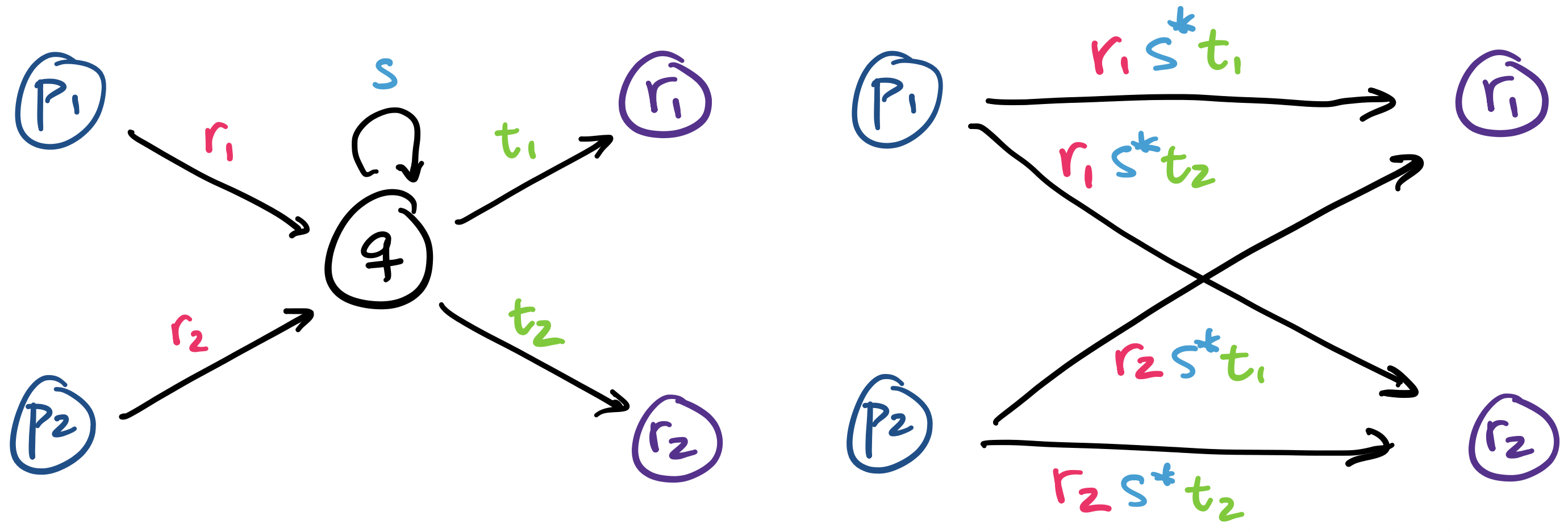
Technically, this alternative algorithm is called state elimination and is due to Brzozowski and McCluskey in 1963. Rather than do the whole DP treatment, the idea is to systematically remove states and relabel the remaining transitions with regular expressions for the paths that travel through the eliminated state. Basically, when we eliminate a state, we replace the transitions to and from the state with regular expressions that represent the strings that would’ve travelled through it. It’s not too hard to see that this is basically what the DP algorithm does, but for all possible pairs of states.
Some texts go through the trouble of formally defining these as “generalized” finite automata, but that’s not really necessary because we’re just using these as a helpful way to keep track of the regular expressions that we’re building and not using them as a real mathematical object. (Now, if you were implementing this, that would be a different story)
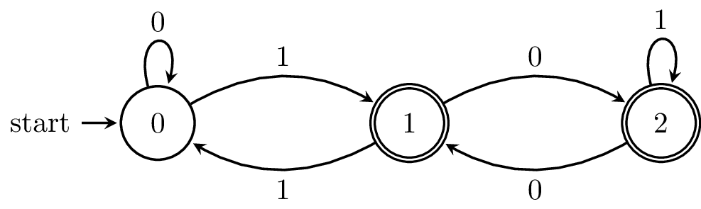
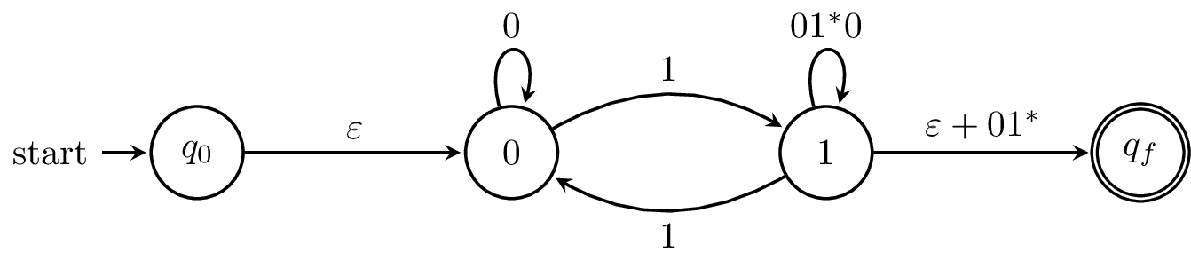
Consider the following DFA, which is the complement of our "divisible by 3" DFA (i.e. the numbers that aren’t divisible by 3).
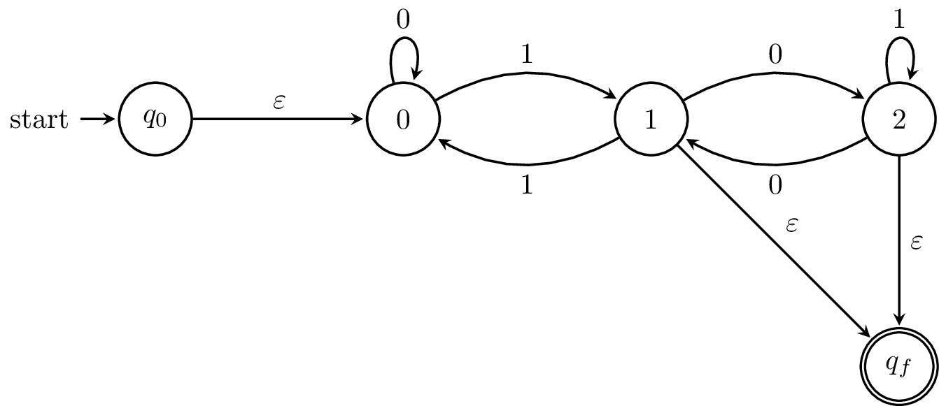
To make things simpler, we begin by adding an initial state and final state and connect $\varepsilon$-transitions as appropriate. Otherwise, we have to contend with the issue of what happens when we try to "eliminate" an initial or final state.
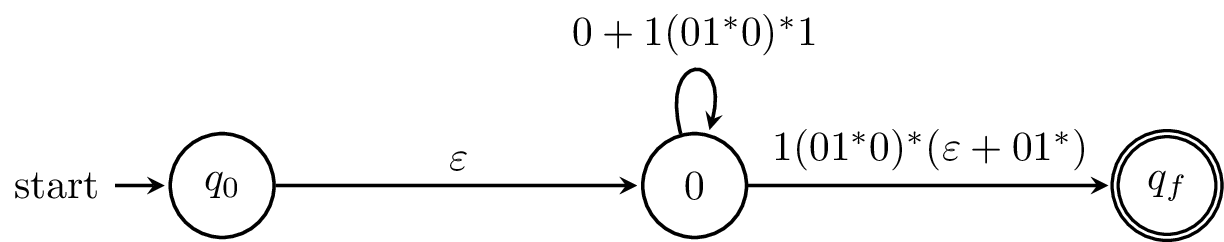
Consider a path from $1$ through $2$ and back to $1$. This is $1$ followed by any number of $0$s and $1$ again. Similarly, if we didn’t go back, we’d be in a final state, so we need to consider that alternative. What this amounts to is figuring out regular expressions for all possible paths through the state we eliminate.
We do this again with all of the states of our original automaton. What we should be left with is a "finite automaton" with a single transition labelled by the regular expression for our language.
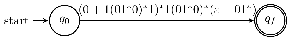
Again, we can see that this process is based on the idea from the DP algorithm, constructing regular expressions for part of the machine and combining them, and with very much the same reasoning. The difference is that we’re not doing this for all possible pairs and paths.
What are some consequences of Kleene’s theorem? One thing you may have noticed about our regular expressions and the regular expressions you’ve used (namely POSIX regular expressions) have different sets of operators that you can use. Can we augment our regular expressions with more operators without changing their power? One easy way to do this is to make use of finite automata to prove closure properties for those operations—if you can construct a DFA for it, then you can add it to your regular expressions without any worry!
This sounds great, but it turns out that there are some features defined in POSIX that aren’t regularity-preserving. In particular, backtracking can allow regexes to describe languages which are not regular. In other words, this feature means that standard Unix/Posix regular expressions aren’t actually regular! A formal study of the power of such “practical” regular expressions was done by Câmpeanu, Salomaa, and Yu in 2003.
Derivatives of Regular Expressions
While we have a pretty good understanding of how a DFA processes a word, we've been comparatively vague about how to think about the same process when matching a word against a regular expression. For example, how would we talk about a word that has partially matched a regular expression, in the same way that we could think about a DFA that's halfway through reading a word?
Suppose we have a regular expression $\mathtt{b(a+b)^*b}$ and I have the first letter of a word, $b$. I want to know what the possible matches are after I have read/matched a $b$. For this expression, it is easy to tell: it is anything that ends with a $b$. But we can also use our regular expression to describe this set: it is the original expression without the first factor, $\mathtt{(a+b)^*b}$.
This idea of a regular expression describing the set of strings after a partial match is called a derivative of the regular expression. We can think of derivatives in the sense that we'll be considering a regular expression after it has partially matched a word, or capturing how the expression changes as it matches a word.
Since this is a set of strings, it's a language. What does this language look like?
The quotient of a language $L$ by a word $w$ is the language
$$w^{-1} L = \{x \in \Sigma^* \mid wx \in L\}.$$
Much like how ideas like concatenation, powers, and factors (subwords) invoke analogies to multiplication, the use of the term quotient in this case can be thought of in the same way. The quotient $w^{-1} L$ is what's left when we "factor out" $w$ from the front of the word.
Note that we can take quotients on any language, not just those that are regular. However, a key observation that Janusz Brzozowski made in 1964 was that one can compute a quotient for a regular language via its regular expression. This is the genesis of the derivative.
First, we define the notion of the constant term of a regular expression.
The constant term of a regular expression $\mathbf r$, denoted $\mathsf c(\mathbf r)$, is defined by
\begin{align*}
\mathsf c(\varnothing) &= \varnothing, & \mathsf c(\epsilon) &= \epsilon, &\mathsf c(\mathtt a) &= \varnothing \text{ for all $a \in \Sigma$},
\end{align*}
and for regular expressions $\mathbf r_1$ and $\mathbf r_2$,
\begin{align*}
\mathsf c(\mathbf r_1 + \mathbf r_2) &= \mathsf c(\mathbf r_1) + \mathsf c(\mathbf r_2), & \mathsf c(\mathbf r_1 \mathbf r_2) &= \mathsf c(\mathbf r_1)\mathsf c(\mathbf r_2), & \mathsf c(\mathbf r_1^*) &= \epsilon.
\end{align*}
The consequence of this definition can be summed up as follows.
For a regular expression $\mathbf r$,
$$\mathsf c(\mathbf r) = \begin{cases} \epsilon & \text{if $\varepsilon \in L(\mathbf r)$,} \\ \varnothing & \text{if $\varepsilon \not \in L(\mathbf r)$,} \end{cases}$$
and therefore, $L(\mathsf c(\mathbf r)) = L(\mathbf r) \cap \{\varepsilon\}$.
This makes for a nice exercise to prove, just do it by induction on $\mathbf r$. In short, the constant term of $\mathbf r$ acts as an “indicator” for whether $\varepsilon$ is in the language of $\mathbf r$.
Observe that the result of $\mathsf c(\mathbf r)$ is a regular expression: it is either $\epsilon$ or $\varnothing$, depending on whether or not $\varepsilon$ is matched by $\mathbf r$ (i.e. whether $\varepsilon$ is a member of the language of $\mathbf r$).
Let's consider the constant term of $\mathbf r = \mathtt{b(a+b)^*b}$. From the above proposition, this should be $\varnothing$, since $\varepsilon \not \in L(\mathbf r)$. According to the definition, we have
\begin{align*}
\mathsf c(\mathtt{b(a+b)^*b}) &= \mathsf c(\mathtt b) \cdot \mathsf c(\mathtt{(a+b)^*b}) \\
&= \varnothing \cdot \mathsf c(\mathtt{(a+b)^*b}) \\
&= \varnothing
\end{align*}
What is neat about this is that it can be used as a “switch” in regular expressions that will activate different subexpressions depending on the presence of $\varepsilon$ in the language. The benefit of this definition is that it’s completely mechanical and computable by rolling out the definition and applying the rules of algebra.
Why is $\mathsf c$ called the constant term? If we recall the regular expressions as an algebra, then we can think of $\varnothing$ as the "0" (additive identity) and $\epsilon$ as the "1" (multiplicative identity) of the regular expressions. In this way, they are the constants.
Now, we are ready to define the derivative of a regular expression, which is itself a regular expression.
Let $\mathbf r$ be a regular expression. Then the derivative of $\mathbf r$ with respect to $a \in \Sigma$, denoted $\frac{d}{da}\mathbf r$, is defined recursively by
\begin{align*}
\frac{d}{da}\mathtt a &= \epsilon,
&\frac{d}{da}\mathtt b &= \varnothing \text{ for $b \in \Sigma$ and $b \neq a$},
&\frac{d}{da}\epsilon &= \varnothing,
&\frac{d}{da}\varnothing &= \varnothing,
\end{align*}
and for regular expressions $\mathbf r_1$ and $\mathbf r_2$,
\begin{align*}
&\frac{d}{da}\left(\mathbf r_1 + \mathbf r_2\right) =& \frac{d}{da}\mathbf r_1 + \frac{d}{da}\mathbf r_2,& \\
&\frac{d}{da}\mathbf r_1\mathbf r_2 =& \left(\frac{d}{da}\mathbf r_1\right) \mathbf r_2 + \mathsf c\left(\mathbf r_1\right) \frac{d}{da}\mathbf r_2,& \text{ and } \\
&\frac{d}{da}\mathbf r_1^* =& \left(\frac{d}{da}\mathbf r_1\right) \mathbf r_1^*.&
\end{align*}
You might think this notation is kind of cute because it evokes the idea of derivatives from calculus. This notation is based on the $\partial$ notation of Jacques Sakarovitch, in Elements of Automata Theory. I prefer it to the $D_a$ notation from the original Brzozowski paper.
The definition of the derivative gives us a way to compute a regular expression $\frac{d}{da} \mathbf r$, given some regular expression $\mathbf r$ and symbol $a \in \Sigma$. The claim here is that this regular expression describes all words $x$ such that $ax$ was matched by $\mathbf r$. In other words, the language of the derivative $\frac{d}{da}\mathbf r$ should be exactly the quotient $a^{-1}L(\mathbf r)$. This is a claim that requires proof.