Unrestricted grammars
Earlier, we saw from the Chomsky hierarchy that the Type-0 or unrestricted grammars are those grammars that generate exactly the Turing-recognizable languages. We will try to work through this result.
We’ve seen already that Turing machine configurations can be represented using strings. We’ve also seen that rewriting a configuration into the configuration that follows from an application of the transition function actually isn’t that hard: we just have to find the state indicator and make the appropriate changes. This actually turns out to be relatively straightforward with a grammar.
For instance, for each transition $\delta(p,X) = (q,Y,\rightarrow)$, we know that this corresponds to the computation step $upXv \vdash uYqv$. With an unrestricted grammar, this can be represented as the rule $pX \to Yq$. Similarly, for $\delta(p,X) = (q,Y,\leftarrow)$, this looks like $uZpXv \vdash uqZYv$, which would be represented using the rule $ZpX \to qZY$, thoug we have to account for all possible $Z \in \Gamma$ since we’re moving to the left.
From this, it’s not hard to see that we can encode the transition function $\delta$ of a Turing machine as rules of an unrestricted grammar. Once we have these rules, we can then transform a starting configuration $q_0 w$ to some accepting configuration $u q_{\mathsf{acc}} v$. This accounts for most of the main “intellectual” core of the idea. What remains is a bit more technical.
Basically, there are two main problems to resolve, having to do with the core differences between the Turing machine and unrestricted grammar models.
- Turing machines are mechanisms that read an input string and answer Yes or No, while grammars are mechanisms that generate strings. The grammar we just described is not complete, since we only described how to start with some initial configuration of a Turing machine and end with an accepting configuration. This is not the same as generating a string from the language accepted by the Turing machine.
- Turing machines are deterministic, while grammars are nondeterministic.
So any proof of equivalence must bridge these two gaps. We’ll start with the issue of nondeterminism.
Nondeterminism and simulating other models
What we will try to do is define the notion of a nondeterministic Turing machine and then show that such a machine can be simulated using our ordinary deterministic Turing machine.
We’ve seen already that the Turing machine model is quite robust to changes. For instance, we discussed the notion of computable functions, for which the notion of acceptance and rejection doesn’t really make sense. In this case, one can modify the Turing machine so that instead of having an accepting or rejecting state, we have a halting state. This model is equivalent since we can interpret an output of $0$ to be “reject” and $1$ to be “accept”.
Another observation is that even the basic definition has variants:
- Some models allow for the tape head to “stay” rather than move left or right on a transition.
- Some models define only a set of explicit accepting states, as in DFAs, NFAs, and PDAs, with rejection implicitly defined via undefined transitions.
- Some models define the tape to have a left “end” and infinite to the right, while some models define the tape to be infinite in both directions.
We’ve also seen specialized machines, like the enumeration machine that takes no input, but lists all the strings in some Turing-recognizable language.
It is not hard to see that all of these models can be simulated by the basic Turing machine model (whichever one we decide on). Just like with DFAs and PDAs, it is worth asking what kinds of modifications we can make and still retain the same “power” of the machine.
One example of how we can modify the Turing machine model is to ask what if instead of using only a single tape, we allowed the Turing machine to have multiple tapes with tape heads that move independently of each other? That is, for $k$ tapes, we modify the definition so we have the transition function $\delta : Q \times \Gamma^k \to Q \times \Gamma^k \times \{L,R\}^k$.
Every language recognized by a multi-tape Turing machine can be recognized by a single tape Turing machine.
In fact, we’ve already seen this kind of idea when discussing the universal Turing machine. For that machine, we discussed a scheme to “divide” the tape. The idea of representing $k$ tapes proceeds much along the same lines.
We show how to simulate a multi-tape Turing machine on a single-tape Turing machine. The idea is to store all the contents of each tape on the single tape and separate each tape as required. We also keep track of the tape head positions on each of the virtual tapes.
What does this machine look like? We describe a Turing machine which simulates a $k$-tape TM $M$ as follows:
- On input $w = a_1 \cdots w_n$: Format the tape so that it represents the $k$ tapes of $M$ by
$$\# \dot a_1 a_2 \cdots a_n \# \dot \Box \# \dot \Box \# \cdots \#$$
- To simulate a single move, scan the tape from the first $\#$, which marks the left hand end, to the $(k+1)$st $\#$, which marks the right hand end to determine the symbols under the virutal tape heads. Make another pass to update the tape heads according to the transition function of $M$.
- If a virtual tape head gets moved to the right onto a $\#$, this means that $M$ moved the corresponding tape head onto a blank portion of the tape. We write a $\Box$ on this tape cell and shift the contents of the rest of the tape to the right and continue the simulation.
Since a single-tape Turing machine can obviously be simulated by a $k$-tape Turing machine, this tells us that the two models are equivalent.
Now, based on what we’ve discussed, the $k$-tape machine is really a convenience for us to think about how the machine stores information. As discussed in the proof, we could have accomplished this in the way we’ve been doing all along, by talking about reserved portions of the tape. In any case, we can now make use of this model to discuss how to simulate nondeterminism.
First, what does a nondeterministic Turing machine look like? In a nondeterministic Turing machine, the transition function is a function $\delta: Q \times \Gamma \to 2^{Q \times \Gamma \times \{L,R\}}$. That is, our transition function maps onto a set of possible transitions.
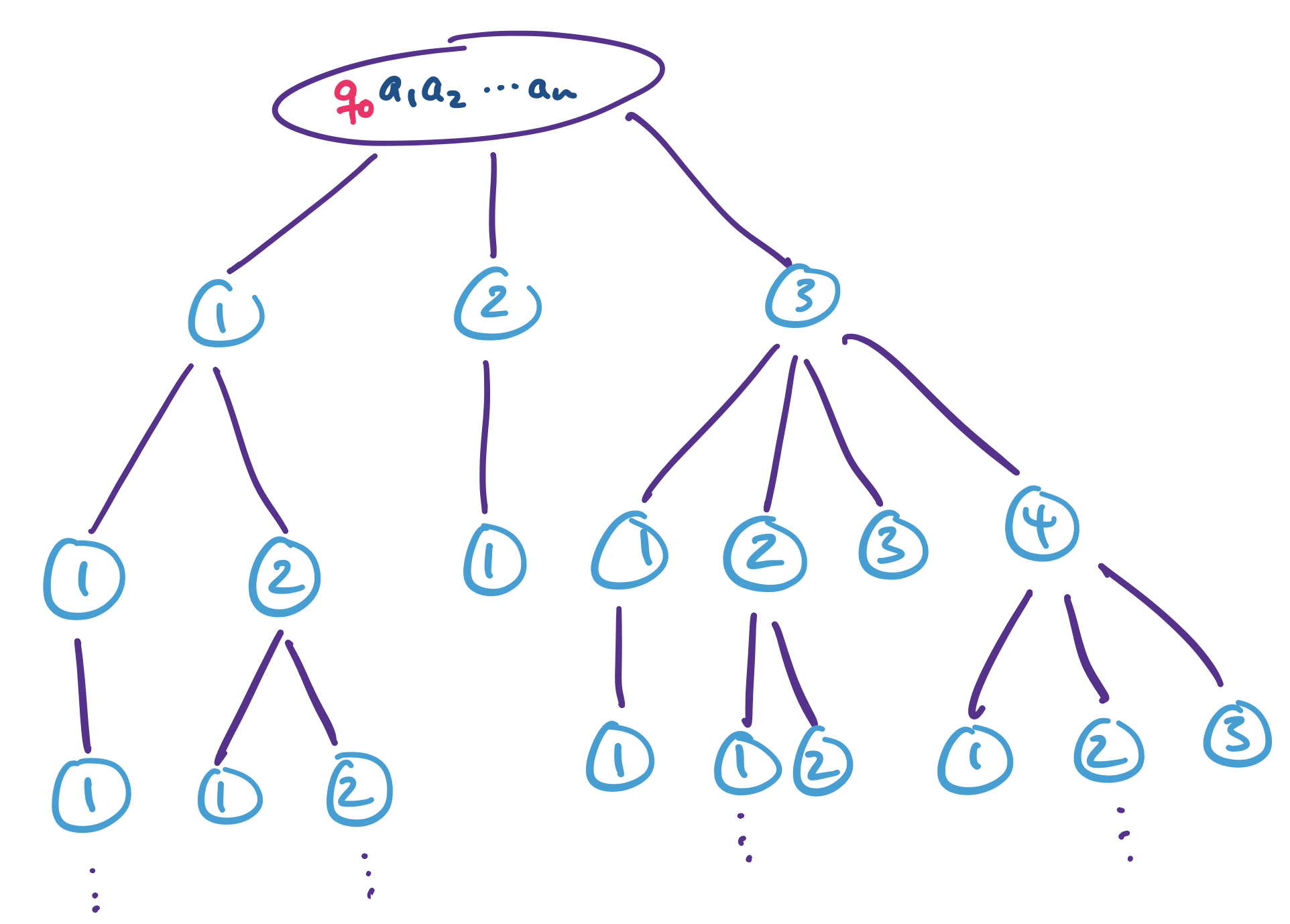
As with other nondeterministic models, we can view the computation of a nondeterministic Turing machine as a tree, where each branch represents a possible choice or guess. Then a nondeterministic Turing machine accepts a word if at least one branch of the computation tree enters an accepting state. It’s important to note that, as with other nondeterministic models, a nondeterministic Turing machine $M$ on an input string $w$
- accepts $w$ if at least one branch of computation reaches an accepting configuration, and it
- rejects $w$ if every branch of computation reaches a rejecting configuration.
Every nondeterministic Turing machine has an equivalent deterministic Turing machine.
The idea behind this proof is to construct a Turing machine that performs a breadth-first search of the computation tree. Recall that the transition function of a nondeterministic Turing machine is a function $\delta: Q \times \Gamma \to 2^{Q \times \Gamma \times \{\leftarrow, \rightarrow\}}$. Since $Q$ and $\Gamma$ are both finite, any single transition has a finite number of choices, so every node in the tree is guaranteed to have finitely many children.
Since we do a breadth-first search, if the machine accepts the input string, the branch containing an accepting configuration will be finite and we will eventually find it. Similarly, if the machine rejects the input string, we will eventually find all rejecting configurations. And if the machine runs forever, then the search will continue forever.
We use a 3-tape deterministic machine to simulate the nondeterministic machine $N$. We can do this because we have just conveniently showed that a $k$-tape machine is equivalent to a single tape machine. The tapes are used as follows:
- The first tape keeps a copy of the input word at all times.
- The second tape is an instance of $N$’s tape on a branch of computation.
- The third tape is an “address” that points to a particular configuration in the computation tree of $N$.
The third tape is what will allow us to navigate through the tree. Let $k = \max\limits_{q \in Q, a \in \Gamma} |\delta(q,a)|$. This is the largest number of choices for any single transition in the machine. For each node, we assign a value to each child from $1$ to $k$. Then by considering a string over the alphabet $\{1,\dots,k\}$, we follow a particular branch at each set of choices, starting from the root of the tree.
Note that not every string over $\{1,\dots,k\}$ will correspond to a valid address, since not every nondeterministic set of choices is guaranteed to have as many as $k$ choices. But this is fine, since that address simply will not correspond to a node. Then by enumerating through every string, we are guaranteed to reach every node of the computation tree.
Now, the machine operates as follows:
- Initialize the tapes so that tape 1 contains the input word $w$, tape 2 begins with a copy of $w$ and 3 is set to $\varepsilon$.
- Use tape 2 to simulate $N$ on $w$. At each step, check the next symbol on tape 3 to determine which choice to make on the transition function of $N$. If no more symbols remain on tape 3 or if the choice is invalid, abort the branch and move to the next stage. If a rejecting configuration is encountered, move to stage 3. If an accepting configuration is encountered, accept.
- Increment the string on tape 3, copy the input $w$ from tape 1 to tape 2, and move to stage 2 to begin simulation of the next branch of computation.
Something you might notice or object to is that simulating a nondeterministic Turing machine with a deterministic machine can potentially take a very long time. Since we’re performing a breadth-first search, this means that we’re looking at a computation that’s exponential in the length of the shortest accepting path in the nondeterministic computation tree. But that’s okay, because we only care whether our deterministic machine is able to recognize or decide any language that a nondeterministic machine is capable of recognizing.
But for argument’s sake, let’s suppose that we do care about the time that it takes. We can measure this: how many steps is the computation on our machine? We can apply our notions of efficiency from other CS courses and consider polynomially many steps to be good or efficient. So suppose that I have a nondeterministic TM that has an accepting computation branch that’s polynomially long in the size of the input. Is it possible to simulate or come up with a way to solve the same problem deterministically, but still end up with only a polynomially long computation?
The answer is: we don’t know! Because this question is exactly the P vs. NP problem.
Machine and grammar simulations
Since we now know that nondeterministic and deterministic Turing machines are equivalent, we can use a nondeterministic machine as our basis for discussion and take advantage of nondeterminism. This will make it much easier to think through how the operation of the machine aligns with the behaviour of the grammar.
We’ll start with the easier case: given an unrestricted grammar, show that a Turing machine can recognize the language of the grammar.
Let $G = (V, \Sigma, P, S)$ be an unrestricted grammar. Then $L(G)$ is Turing-recognizable.
Construct a nondeterministic Turing machine that does the following:
- On input string $w$, set up four tapes so that it holds the following information:
- the input string $w$ (this tape does not change),
- a sentential form,
- the left hand side of a production, and
- the right hand side of the same production.
- Initialize the sentential form to $S$, the start variable.
- Nondeterministically choose a cell on the sentential form tape.
- Nondeterministcally choose a production and write the rule to the reserved locations.
- If the selected location on the sentential form tape matches the left hand side of the chosen production, replace the corresponding symbols on the sentential form tape with the right hand side of the chosen production.
- Repeat this process until the sentential form matches the input tape, and accept.
Recall that when generating a string using a grammar, there are two possible nondeterministic choices for each step of a derivation:
- which part of the sentential form to rewrite, and
- which production rule to apply.
We use a nondeterministic machine to handle these two choices. The result is a machine that nondeterministically applies productions. If $w$ is a string that is generated by $G$, there must exist a derivation $S \Rightarrow^* w$ in $G$ and so there must exist a series of nondeterministic choices that our Turing machine can apply. So our machine will accept the string.
On the other hand, if $G$ does not generate $w$, then there will be no series of choices that our machine will apply that generates $w$. In this case, the machine will either run out of possible rules to apply or run forever. In either of these case, the machine does not accept $w$.
Showing that a Turing machine can simulate a grammar turned out not to be too difficult, by taking advantge of the ability of a Turing machine to write strings and nondeterministically choose strings for granted. What is less obvious is showing that a grammar can simulate a Turing machine.
One way to do this is to meet in the middle: instead of simulating a Turing machine that accepts a language, we instead simulate a Turing machine that nondeterministically generates a string from the language. This is not too different from how we defined a Turing machine that enumerates all strings from a language.
Let $L$ be a Turing-recognizable language. Then there exists an unrestricted grammar $G$ such that $L(G) = L$.
Let $M$ be a Turing machine that recognizes $L$. Using $M$, we construct a nondeterministic Turing machine $M'$ that nondeterministically “generates” a string from $L$ in the following way:
- Nondeterministically choose a string $w \in \Sigma^*$.
- Copy $w$ to a reserved portion of the tape.
- Simulate $M$ on input $w$ on the work portion of the tape.
- If $M$ accepts $w$, erase the work portion of the tape and halt, leaving $w$ on the tape.
One way to think about this machine is that for each string $w \in L$, there is a branch of computation that successfully simulates a computation of $w$ on $M$ and ends with $w$ remaining on the tape. For strings $w \not \in L$, there will be no successful computations of $M$ on $w$ so these will either crash/reject or run forever.
One issue here is how to handle the erasing of the work tape in the final step. This issue arises if $M$ ever writes blanks—we need to get rid of any that our machine wrote but not the infinitely many that our machine never encountered. The trick is to make sure that $M'$ never writes a blank ($\Box$) to the tape by making it write something like $\boxdot$ instead. This way, we can distinguish truly blank tape cells and cells in which we’ve overwritten and we don’t try to erase the infinitely many blank cells that were never visited.
Based on this, we can construct the following grammar to simulate $M'$, the nondeterministic generator for $L$.
\begin{align*}
S &\to q_0 S_1 \\
S_1 &\to \Box S_1 \mid T \\
pX &\to Yq &\text{for each $(q,Y,\rightarrow) \in \delta(p,X)$} \\
ZpX &\to qZY &\text{for each $Z \in \Gamma$ and $(q,Y,\leftarrow) \in \delta(p,X)$} \\
q_{\mathsf{acc}} \boxdot &\to q_{\mathsf{acc}} \\
q_{\mathsf{acc}} \Box &\to q_{\mathsf{acc}} \\
q_{\mathsf{acc}}T &\to \varepsilon
\end{align*}
We can split these rules up into three groups:
- The productions on $S$ and $S_1$ describe the initialization phase of a derivation. A derivation begins with $S \Rightarrow^* q_0 \Box^n T$ for some $n$ with $T$ as an endmarker. Notice that $q_0 \Box^n$ is an initial configuration.
- The next two lines describe rules that correspond to transitions $\delta$ of the Turing machine. These allow our grammar to simulate a Turing machine computation by manipulating the configuration.
- At some point, a configuration with $q_{\mathsf{acc}}$ is reached. The last three rules describe the tape erasure phase. Recall that we assume the machine we’re simulating is the nondeterministic TM that generates a string. We assume that at the point the accepting configuration is reached, the tape head is at the right of $w$ and on top of a blank. At this point, the rules to erase the remaining blanks are applied and we are left with $w$.
The equivalence of unrestricted grammars and Turing machines ties a nice bow on many ideas we’ve seen throughout the quarter.
- This is another example of the equivalence between a machine model and a grammar, in the same way we saw for regular languages and context-free languages. This is only one equivalence out of many other different models (the same is true of regular and context-free languages).
- This equivalence works via simulation. The Turing machine is able to simulate the action of the grammar, while the grammar simulates the action of the Turing machine.
- Turing machines are a convenient model for representing the power of computation. In showing equivalence, we’ve shown that unrestricted grammars are a model that can also represent the full power of computation.
- Computation can ultimately be reduced to string rewriting and manipulation. The equivalence of Turing machines with unrestricted grammars shows that we can carry out a computation simply through rewriting a string.
One observation about this is that very little machinery is actually required for computation. The Turing machine and unrestricted grammar models are not extremely complicated. They actually have fairly small, well-defined sets of rules. Despite this, they can express the full power of computation. This is one of the surprising consequences of the Church–Turing thesis and why it’s easy to run into mechanisms that can perform computation. In this sense, it is a bit surprising that we’ve basically hit the limits of computation even on relatively simple systems.
Computation is just strings, which is why computation is everywhere, but we still can’t compute everything.