Let’s go back to concatenation and define a few more notions.
We will often need a way to express repetition of concatenation. One way to do this is via “powers”. This works the way that you would expect it to work.
The $k$th power of a string $w$ is $$w^k = \overbrace{ww \cdots w}^{k \text{ times}}$$ and we define $w^0 = \varepsilon$. Formally, we define this inductively by
Notice that this definition is inductive on the natural numbers rather than strings.
We often see “power”-like terms used to describe certain kinds of strings as well. For example, a string that is of the form $w = x^2$, like $catcat$ where $x = cat$, is called a square and a string of the form $w = x^3$ like $hohoho$, where $x = ho$, is called a cube.
A related notion that won’t come up very much in this course is the notion of primitivity. We say a word is primitive if it is non-empty and can’t be written as the power of some other word. This is sort of like the notion of a “prime unit” for strings.
Something else that we will often be interested in is talking about parts of a string.
If $w = uxv$ is a string, we say
It’s important to note that $u,v,w,x$ are strings, which can include $\varepsilon$. So, for instance, we can say that $\varepsilon$ is a prefix of every string and that $w$ itself is a prefix of $w$.
Let $w = cat$.
Much like the usage of “string” or “word”, there are a plethora of terms that can be used interchangeably to describe what you’re probably most familiar with as a substring. The term subword is the same idea, if you were to use word instead of string. Similarly, the term infix comes naturally from the analogy with prefix and suffix. The one which may be less obvious is factor; this comes from viewing the string as an algebraic object: if $6 = 1 \times 2 \times 3$, then $2$ is a factor of $6$. Similarly, if $w = x \cdot y \cdot z$, then $y$ is a factor of $w$.
Again, the choice of which term to use is largely a product of which subfield you spend your time in (computer science, combinatorics, or algebra) and where you are situated geographically (the Americas or Europe).
Because string concatenation is not commutative (i.e. $uv$ is not necessarily the same as $vu$), we can think of strings as having a “direction”, being read from left to right. This means that there is a notion of reversing a string.
The reversal of a string $w = a_1 a_2 \cdots a_n$ is the string with the symbols written in reverse order, $w^R = a_n \cdots a_2 a_1$. Formally,
If $w = w^R$, we say $w$ is a palindrome.
As we’ve seen earlier, languages in the formal language theoretic sense are just sets of strings and we describe a language in the same way as for any other set.
Here are some examples of languages.
We can define the notion of a language a bit more formally, with respect to an alphabet $\Sigma$.
We denote by $\Sigma^*$ the set of all finite words over the alphabet $\Sigma$. A language $L$ over $\Sigma$ is a subset $L \subseteq \Sigma^*$.
In other words, we fix some alphabet $\Sigma$ and take $\Sigma^*$ to be our universe.
By finite words, we mean words of finite length. One can define a notion of infinite strings, but we won’t be dealing with those in this course. Also keep in mind that languages are sets and sets can have infinite cardinality (this is what makes things difficult).
You might notice that the more curious definition is for $\Sigma^*$. If you recall our brief diversion about monoids, you might recognize that $\Sigma^*$ is really just the free monoid on $\Sigma$.
Since languages are sets, we can perform any set theoretic operations we’re familiar with, like union and intersection. In the case of complement, since we have an explicit universe, we get the following definition.
For a language $L \subseteq \Sigma^*$, the complement of $L$ is $\overline L = \Sigma^* \setminus L$.
This also means there are a few things we have to be careful with. For example, there is the notion of the empty language $\emptyset$, which is the language with no strings in it. This is different from the language $\{\varepsilon\}$, which is the language containing the empty string.
We can also extend many operations on strings to operations on languages.
For two languages $L_1$ and $L_2$, we define the catenation of $L_1$ and $L_2$ by $$ L_1 L_2 = \{uv \mid u \in L_1, v \in L_2 \}.$$
If $L_1 = \{\varepsilon, ab, abb, abc\}$ and $L_2 = \{ca, bac\}$, then \[L_1 L_2 = \{ca, bac, abca, abbac, abbca, abbbac, abcca, abcbac\}.\] Notice that like the definition of concatenation on strings, the order in which two languages are concatenated matters.
What exactly is the difference between $\emptyset$ and $\{\varepsilon\}$? Concatenation gives us one example of why this difference matters. Consider a language $L$ and the following languages:
One way to think about concatenation is as taking the cartesian product of two sets and then “flattening” the resulting tuples.
        >>> from itertools import product
        >>> concat = lambda L, M: {''.join(x) for x in product(L, M)}
        >>> L1 = {'', 'ab', 'abb', 'abc'}
        >>> L2 = {'ca', 'bac'}
        >>> concat(L1, L2)
        {'abbac', 'abbbac', 'abbca', 'abca', 'abcbac', 'abcca', 'bac', 'ca'}
        >>> concat(L1, {''})
        {'', 'ab', 'abb', 'abc'}
        >>> concat(L1, set())
        set()
Notice that the language $\{\varepsilon\}$ acts as an identity for concatenation on languages the same way that $\varepsilon$ does for strings. This gives us a way to define powers for languages.
For a language $L \subseteq \Sigma^*$, the $k$th power of $L$ is
This definition leads to a very important definition in formal language theory.
Let $L = \{ab, abb, abc\}$. Then
and so on.
        >>> from itertools import product
        >>> power = lambda L, k: {''.join(x) for x in product(L, repeat=k)}
        >>> L = {'ab', 'abb', 'abc'}
        >>> power(L,0)
        {''}
        >>> power(L,1)
        {'ab', 'abc', 'abb'}
        >>> power(L,2)
        {'abbab', 'ababc', 'abbabc', 'abbabb', 'ababb', 'abcabb', 'abcab',
        'abcabc', 'abab'}
        >>> power(L,3)
        {'abbababb', 'abababb', 'abbabbabc', 'abbabbabb', 'abcababc',
        'abcabbab', 'abbabcab', 'abcababb', 'abcabbabc', 'abcabbabb',
        'abcabcabb', 'abbabcabb', 'abcabcab', 'ababcab', 'abbabcabc',
        'ababab', 'ababbabc', 'ababcabb', 'abbabab', 'abcabcabc', 'ababbab',
        'ababbabb', 'ababcabc', 'abbababc', 'abbabbab', 'abcabab', 'abababc'}
This definition leads to a very important definition in formal language theory.
The Kleene star or Kleene closure of $L$ is defined by $$ L^* = \bigcup_{i \geq 0} L^i.$$ We define the positive Kleene closure of $L$ by $L^+ = LL^*$. One can see that this is just the nonzero powers of $L$, so we can also think of this as $$ L^+ = \bigcup_{i \geq 1} L^i.$$
Here closure is meant as closure of the set under concatenation. Observe that of all the operations we’ve seen, the Kleene star is the one that allows us to define infinite sets.
Let $\Sigma = \{a,b,c\}$. Then $L = \{ab, bc\}$ is a language over $\Sigma$. If we take the Kleene star of $L$, we get the language made of up of combinations of $ab$ and $bc$: \[\varepsilon, ab, bc, abab, abbc, bcab, bcbc, ababab, ababbc, abbcab, abbcbc, bcabab, bcbcab, \dots\]
One use of this is for constructing codes. In formal language theory, a code over an alphabet $\Sigma$ is a language $K \subseteq \Sigma^+$ such that if $w \in K^+$ then $w$ has a unique factorization into words of $K$ (here is a use of “factor” as “subword”). It’s not hard to see that not every language is a code.
For example, our language $L$ above is a code (try to explain why). However, the language $\{ab, abb, ba, bb\}$ is not a code since the string $abbabb$ can be decomposed into $ab \cdot ba \cdot bb$ and $abb \cdot abb$.
Computer science and the theory of computation emerged from the big questions of mathematical logic in the early 20th century. The machines that we rely on called computers did not exist and would not really exist for about another forty to fifty years. But even back then, the notion of computation was still tied to a model or machine. The model would define the finite set of operations or instructions it could execute. One of the big questions early on was figuring out which model was the right one.
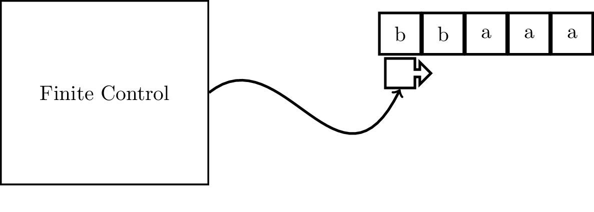
The model that we will be focusing on in this course and the one that arguably “won” in terms of being the broadly accepted model of computation is due to Alan Turing in 1936, known now as a Turing machine. A Turing machine has an input tape, divided into cells, with an input word written on it. The machine has a tape head that can scan the input tape, reading a symbol from each cell. The machine is also equipped with a finite set of instructions that will tell the machine how to act based on what it reads off of the tape. This set of instructions is represented as a set of states.
The machine will read one tape cell, and therefore one symbol, at a time. Based on what it reads and the state that the machine is in, it will do the following:
What exactly does this model try to capture? What Turing attempted to do was formalize how computers worked, by which we mean the 1930s conception of what a computer is. In other words, he tried to formalize how human “computers” might “compute” a problem. We can view the finite state system as a set of instructions we might give to a person, that tells them what to do when they read a particular symbol. We allow this person to read and write on some paper and we let them have as much paper as they want.
Here, we should stop a bit and discuss the right analogy for the notion of a “machine”. It’s tempting to think of this as a model of a general-purpose, programmable computer because that’s what we imagine when we hear “machine”. However, this is not necessarily what mathematicians in the early 20th century were imagining.
Recall what we are trying to do: we are trying to define a “machine” that will solve a problem. A problem is a set of strings, so a machine, when given an input string, tells us whether the string is in the set or not. This is a solution to the problem. But problems are functions and solutions to these kinds of problems are algorithms.
So the right metaphor is that machines are really algorithms, not computers. In modern algorithms, we imagine an algorithm as a sequence of operations that we agree are “basic”. Here, the operation that is allowed is the “read-check state-write-move” cycle and the states and transitions are the “sequence of operations”.
Instead of jumping into working with the full model we described, we will start off by considering the most simplified model, where the machine can only read off of the tape (that is, it can’t write) and it can only scan to the right—the tape head can never move to the left. This simplified model is what is called a finite automaton.
What kinds of problems can be solved in this way? That is, we make exactly one pass through a string and are only able to retain a fixed amount of information. This sounds a lot like (sub)string search: given a text $T$ and a string $w$, does $T$ contain $w$ as a substring?
Suppose we want to determine whether the string $cat$ appears in our text. What information do we need to keep track of? Well, we would want to know whether we’ve seen a $c$, then an $a$, then a $t$. So once we see a $c$, we have to remember that a $c$ was just read. Then what we do depends on the following symbol—whether we see an $a$ or not.
If we flesh this out, we should find that we really need to detect these “states” of whether we’ve seen the right sequence of symbols at any time. More specifically:
This ends up looking like a flow chart, starting from the left and following the arrows depending on the symbol we read.
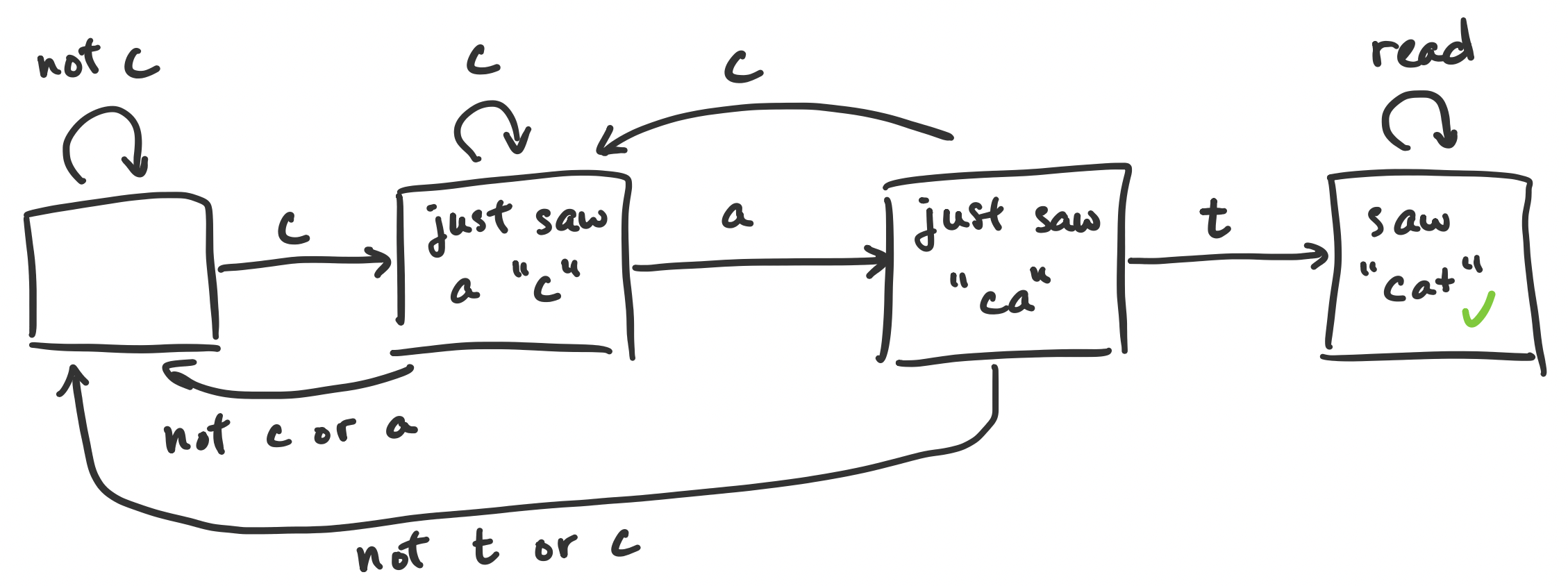
Notice the different possible transitions: if we are “further along” and read a symbol that we’re not interested in, we jump back to the start. Similarly, if at any time we see a $c$, we get put into “just saw a $c$” mode.
This ends up being the basic idea behind finite automata: we have a bunch of states that we transition between based on each symbol of our input string we read. The states represent the possible states of our computation, which work as a very primitive sort of “memory”. In order to say more interesting things about this, we will need to formalize this.