Recognition for grammars
We have seen that grammars are typically used to define the structure of programming languages. However, we do not really have a clear way to determine whether a string is generated by a given grammar $G$—that is, the string is “valid” with respect to the grammar. For an aribtrary CFG, it’s not clear where to even begin with this.
One way to think about this is to think back to the correspondence between regular expressions and finite automata. There, we had a convenient descriptive formalism in the regular expressions which we can transform into a convenient recognizer in finite automata.
Let $G$ be a context-free grammar. Then there exists a pushdown automaton $M$ such that $N(M) = L(G)$.
Let $G = (V,\Sigma,P,S)$ be a CFG. We will create a PDA $M = (Q,\Sigma,\Gamma, \delta, q_0, Z_0)$ which accepts by empty stack defined as follows:
- $Q = \{q\}$,
- $\Gamma = V \cup \Sigma$,
- $q_0 = q$,
- $Z_0 = S$,
and we define the following transitions
- $\delta(q,\varepsilon,A) = \{(q,\alpha) \mid A \to \alpha \in P\}$ for each variable $A \in V$,
- $\delta(q,a,a) = \{(q,\varepsilon)\}$ for each symbol $a \in \Sigma$.
Here is what the machine looks like.
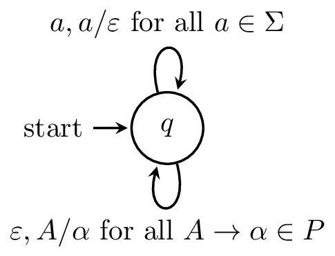
This machine essentially acts as a parser for $G$, albeit a nondeterministic one. Like the one-state machine we saw earlier, the computation in this machine is driven primarily by the stack:
- Whenever we see a variable $A$ at the top of the stack, we pop it and replace it with the right hand side of a production $A \to \alpha$.
- Whenever we see a terminal $a$ at the top of the stack, we pop it and try to consume a symbol of the input word.
This process essentially performs a leftmost derivation of our input word. As usual with a one-state machine, we can elide many of the tricky details of how we can ensure the correct production rule is chosen when we see $A$ through the magic of nondeterminism.
To formally prove this, we need to show that we have a derivation $S \Rightarrow^* w$ over $G$ if and only if there is a computation $(q,w,S) \vdash^* (q,\varepsilon,\varepsilon)$ in $M$.
What is the idea behind this? We can think of this as a recursive descent parser. Generally, recursive descent parsers start with the start variable and try to construct a derivation matching the input string. If it is unsuccessful, it will backtrack and try another option. In essence, we can think of this as a deterministic implementation of a PDA, where we backtrack on the computation tree and try each “nondeterministic choice”. We can also see that the job of the PDA stack ends up being mirrored by the call stack of the parser.
Consider the grammar for palindromes,
$$S \rightarrow aSa \mid bSb \mid a \mid b \mid \varepsilon,$$
and consider a PDA $P$ for this grammar, which we obtain by following the construction of Theorem 17.1. Then a computation of $P$ on the word $aababaa$ looks like
\begin{align*}
(q,aababaa,S) & \vdash (q,aababaa,aSa) \\ & \vdash (q,ababaa,Sa) \\ & \vdash (q,ababaa,aSaa) \\ & \vdash (q,babaa,Saa) \\ & \vdash (q,babaa,bSbaa) \\ & \vdash (q,abaa,Sbaa) \\ & \vdash (q,abaa,abaa) \\ & \vdash (q,baa,baa) \\ & \vdash (q,aa,aa) \\ & \vdash (q,a,a) \\ & \vdash (q,\varepsilon, \varepsilon)
\end{align*}
Here is an implementation.
        from automata.pda.npda import NPDA
        A = NPDA(
            states={0},
            input_symbols=set('ab'),
            stack_symbols=set('Sab'),
            transitions={
                0: {
                    'a': {'a': {(0,'')}},
                    'b': {'b': {(0,'')}},
                    '': {'S': {(0, r) for r in {'aSa', 'bSb', 'a', 'b', ''}}}
                }
            },
            initial_state=0,
            initial_stack_symbol="S",
            final_states=set(),
            acceptance_mode="empty_stack"
        )
And here is a run of the machine that contains all of the configurations that are encountered (something that we would not want to do by hand).
        >>> for i, c in enumerate(A.read_input_stepwise('abba')):
        ...     print(f'Step {i}: {c}')
        Step 0: {PDAConfiguration(0, 'abba', PDAStack(('S',)))}
        Step 1: {PDAConfiguration(0, 'abba', PDAStack(('b',))),
                 PDAConfiguration(0, 'abba', PDAStack(('a',))),
                 PDAConfiguration(0, 'abba', PDAStack(('b', 'S', 'b'))),
                 PDAConfiguration(0, 'abba', PDAStack(())),
                 PDAConfiguration(0, 'abba', PDAStack(('a', 'S', 'a')))}
        Step 2: {PDAConfiguration(0, 'bba', PDAStack(())),
                 PDAConfiguration(0, 'bba', PDAStack(('a', 'S')))}
        Step 3: {PDAConfiguration(0, 'bba', PDAStack(('a', 'a', 'S', 'a'))),
                 PDAConfiguration(0, 'bba', PDAStack(('a', 'b', 'S', 'b'))),
                 PDAConfiguration(0, 'bba', PDAStack(('a',))),
                 PDAConfiguration(0, 'bba', PDAStack(('a', 'b'))),
                 PDAConfiguration(0, 'bba', PDAStack(('a', 'a')))}
        Step 4: {PDAConfiguration(0, 'ba', PDAStack(('a', 'b', 'S'))),
                 PDAConfiguration(0, 'ba', PDAStack(('a',)))}
        Step 5: {PDAConfiguration(0, 'ba', PDAStack(('a', 'b'))),
                 PDAConfiguration(0, 'ba', PDAStack(('a', 'b', 'b', 'S', 'b'))),
                 PDAConfiguration(0, 'ba', PDAStack(('a', 'b', 'b'))),
                 PDAConfiguration(0, 'ba', PDAStack(('a', 'b', 'a'))),
                 PDAConfiguration(0, 'ba', PDAStack(('a', 'b', 'a', 'S', 'a')))}
        Step 6: {PDAConfiguration(0, 'a', PDAStack(('a',))),
                 PDAConfiguration(0, 'a', PDAStack(('a', 'b', 'b', 'S'))),
                 PDAConfiguration(0, 'a', PDAStack(('a', 'b')))}
        Step 7: {PDAConfiguration(0, 'a', PDAStack(('a', 'b', 'b', 'b', 'S', 'b'))),
                 PDAConfiguration(0, '', PDAStack(())),
                 PDAConfiguration(0, 'a', PDAStack(('a', 'b', 'b', 'a', 'S', 'a'))),
                 PDAConfiguration(0, 'a', PDAStack(('a', 'b', 'b'))),
                 PDAConfiguration(0, 'a', PDAStack(('a', 'b', 'b', 'b'))),
                 PDAConfiguration(0, 'a', PDAStack(('a', 'b', 'b', 'a')))}
When given in this form, it’s not clear which configuration in each step leads to the next step. However, we recall that as long as we encounter a configuration with the input consumed and the stack empty, we know we can accept.
Now, we’ll consider the other direction. It turns out we've already done a lot of the work. Recall that we showed that every PDA can be transformed into an equivalent PDA with only one state that accepts by empty stack. Notice also that we happened to create a PDA with one state that accepts by empty stack to parse any given grammar. It turns out we can simply reverse this construction.
Let $P$ be a PDA with one state that accepts by empty stack. Then there exists a grammar $G$ such that $L(G) = N(P)$.
Let $P = ({0}, \Sigma, \Gamma, \delta, 0, Z_0)$. We define $G = (V, \Sigma, P, S)$ by
- $V = \Gamma$,
- $\Sigma$ is the same alphabet,
- $S = Z_0$,
and we define the set of productions $P$ by considering transitions from $\delta$ in the following way: for each transition $(0, Y_1 Y_2 \cdots Y_k) \in \delta(0, a, X)$, we define the production
\[X \to a Y_1 Y_2 \cdots Y_k,\]
where $X, Y_1, \dots, Y_k \in \Gamma$, $a \in \Sigma \cup \{\varepsilon\}$.
An interesting consequence of this reverse construction is that the productions are in "almost" Greibach normal form. From here, we can apply the argument in Kozen Chapter 24 in reverse (this construction, found in Chapter 25, basically says this).
So we have shown that the class of context-free languages (those languages generated by context-free grammars) and the class of pushdown languages (those languages recognized by pushdown automata) are exactly the same. This result is due to Chomsky and Schützenberger and Evey around the same time in 1963.
This is a similar situation as with Kleene’s theorem, where we showed the equivalence of recognizable and regular languages via transformations of finite automata to regular expressions and vice versa. This of course doesn’t say anything directly about the structure of the language. For that, we looked to Myhill–Nerode for regular languages.
For context-free languages, we can turn to, who else, Chomsky and Schützenberger, who, also in 1963, they prove what is now called the Chomsky–Schützenberger theorem.
Every context-free language is a homomorphic image of the intersection of a Dyck language and a regular language.
A proof of this result can be found in Kozen Chapter G.
The Chomsky–Schützenberger theorem tells us that every context-free language can be described by a regular language, a Dyck language, and a homomorphism. The Dyck languages are the family of languages of balanced brackets of $k$ types, named after the combinatorialist Walther von Dyck. Since regular languages are closed under homomorphisms, what this tells us is that context-free languages are “like” regular languages, but what really separates the two is the ability to express “nestedness”, in the sense of brackets or trees.
This aligns with our observations of context-free languages: grammars generate strings in a balanced way, from the inside out, while pushdown automata exhibit nestedness because of the constraints of the stack—it is otherwise just an NFA.
Efficient recognition
Though the PDA construction that we saw leads to the recursive descent parsing algorithm, for general context-free grammars, the possibility of backtracking is still too expensive to use in practice. But this is commonly the case for a lot of problems that we approach recursively at first from the “top-down” perspective. One way to get around this is to consider the problem “bottom-up”.
The top-down approach is natural: start with the “start” variable and try to construct a derivation for the input string. The bottom-up approach is to try to build derivations for each substring of our input string and attempt to piece together those derivations. We can think of this as working “backwards” starting with small pieces and putting them together to get the preceding pieces.
To do this, we can exploit the predictable structure of a CNF grammar to come up with a systematic way of building a derivation. We know that every symbol will have a production that generates it directly and we know that every non-terminal production will have exactly two variables on its right hand side. This means that every derivation of a string longer than a single symbol can be broken up into derivations of exactly two strings.
This naturally gives us some recursive structure to work with. Suppose we have a grammar $G = (V, \Sigma, P, S)$ and a string $w$ that we would like to figure out whether $w \in L(G)$. Recall that this means that $S \Rightarrow^* w$, but as usual, we’ll ask the broader question of whether there exists a variable $A$ such that $A \Rightarrow^* w$. We consider this based on the length of $w$.
- Our base case is when $|w| = 1$. In this case, $w = a$ for some $a \in \Sigma$. There are two options.
- There’s a rule $A \to a$ in $G$.
- There is no such rule.
- What happens when $|w| > 1$? We’ve seen before that we must be in the situation when $w = uv$ where $A \Rightarrow^* w$ implies that $B \Rightarrow^* u$ and $C \Rightarrow^* v$, so we must have $A \Rightarrow BC \Rightarrow^* uv = w$. This means that whether there’s a derivation $A \Rightarrow^* w$ depends on whether there’s a derivation $B \Rightarrow^* u$ and $C \Rightarrow^* v$, so we need to test this for all rules of the form $A \to BC$.
For each string, what we’ll do is remember the set of variables $A$ such that $A \Rightarrow^* w$. Let’s call this set $T(w)$. Our discussion above gives us the folowing recurrence.
\[T(w) = \begin{cases}
\{A \in V \mid A \to w \in P\} & \text{if $|w| = 1$}, \\
\bigcup\limits_{w = uv} \{A \mid A \to BC \in P \wedge B\in T(u) \wedge C \in T(v)\} & \text{if $|w| > 1$}.
\end{cases}\]
We can make this more explicit, for the algorithm, by referring to $u$ and $v$ as indexed substrings of $w = a_1 \cdots a_n$.
\[T(i,j) = \begin{cases}
\{A \in V \mid A \to a_i \in P \} & \text{if $i=j$}, \\
\bigcup\limits_{k=i}^{j-1} \{A \mid A \to BC \in P \wedge B\in T(i,k) \wedge C \in T(k+1,j)\} & \text{if $i < j$}.
\end{cases}\]
This recurrence is a Bellman equation—i.e., a dynamic programming recurrence. This means that what we’ve described is really a dynamic programming algorithm. This algorithm is called the Cocke–Younger–Kasami (CYK) algorithm, named after the three individuals who independently proposed it.
    \begin{algorithmic}
    \PROCEDURE{cyk}{$G = (V,\Sigma,P,S), w=a_1 a_2 \cdots a_n$}
        \FOR{$i$ from 1 to $n$}
            \STATE $T[i,i] = \{A \in V \mid A \to a_i \in P\}$
        \ENDFOR
        \FOR{$m$ from 1 to $n-1$}
            \FOR{$i$ from 1 to $n-m$}
                \STATE $j = i+m$
                \STATE $T[i,j] = \emptyset$
                \FOR{$k$ from 1 to $j-1$}
                    \STATE $T[i,j] = T[i,j] \cup \{A \in V \mid A \to BC \in P \wedge B \in T[i,k] \wedge C \in T[k+1,j]\}$
                \ENDFOR
            \ENDFOR
        \ENDFOR
    \RETURN $S \in T[1,n]$
    \ENDPROCEDURE
    \end{algorithmic}
An interesting feature of this algorithm is how it fills out its “dynamic programming table”. You may be used to algorithms that fill out the table row by row, but here, we’ll see that because we are iterating on the length of the substrings, we end up filling out the table diagonally. This also means that where we need to look for our relevant subproblems is a bit different from the usual dynamic programming algorithms.
Let’s walk through an example of the CYK algorithm.
Consider the following grammar $G$ in CNF.
\begin{align*}
S &\rightarrow BC \mid b \\
A &\rightarrow BC \mid b \\
B &\rightarrow DC \mid BB \mid a \\
C &\rightarrow BA \mid b \\
D &\rightarrow CA \mid c
\end{align*}
We want to determine whether the word $cabab$ is generated by $G$. We will store our results in a table. First, we consider every substring of length 1 and the productions that could have generated each substring. We record which variables are on the left hand side of these productions.
| | $c$ | $a$ | $b$ | $a$ | $b$
|
| | 1 | 2 | 3 | 4 | 5
|
| 1 | $D$ | | | |
|
| 2 | | $B$ | | |
|
| 3 | | | $S,A,C$ | |
|
| 4 | | | | $B$ |
|
| 5 | | | | | $S,A,C$
|
Next, we consider substrings of length 2. A production can generate substrings of length 2 if they lead to two variables that each generate substrings of length 1. For example, we have that entry $1,2$ doesn’t have any variables that can generate it, because there is no production of the form $X \rightarrow DB$. However, we can determine that $ab$ is generated by a production that has either $BA$ or $BC$ on the right hand side. There are such productions: $S \rightarrow BC$, $A \rightarrow BC$, and $C \rightarrow BA$.
| | $c$ | $a$ | $b$ | $a$ | $b$
|
| | 1 | 2 | 3 | 4 | 5
|
| 1 | $D$ | $\emptyset$ | | |
|
| 2 | | $B$ | $S,A,C$ | |
|
| 3 | | | $S,A,C$ | $\emptyset$ |
|
| 4 | | | | $B$ | $S,A,C$
|
| 5 | | | | | $S,A,C$
|
We will now consider substrings of length 3. Here, we have to do a bit more work, because strings of length 3, say $xyz$ can be generated by two variables by $xy$ and $z$ or $x$ and $yz$. We must check both possibilities. For example, for the string $cab$, we can generate it either by $ca$ and $b$ or by $c$ and $ab$. In the first case, $ca$ has no derivation, but the second case gives us a valid derivation, since $ab$ can be generated by $S$, $A$, or $C$ and we have $B \Rightarrow DC \Rightarrow cab$.
| | $c$ | $a$ | $b$ | $a$ | $b$
|
| | 1 | 2 | 3 | 4 | 5
|
| 1 | $D$ | $\emptyset$ | $B$ | |
|
| 2 | | $B$ | $S,A,C$ | $\emptyset$ |
|
| 3 | | | $S,A,C$ | $\emptyset$ | $D$
|
| 4 | | | | $B$ | $S,A,C$
|
| 5 | | | | | $S,A,C$
|
We continue with strings of length 4. Again, we have to consider all of the ways to split up a string of length 4 into two substrings.
| | $c$ | $a$ | $b$ | $a$ | $b$
|
| | 1 | 2 | 3 | 4 | 5
|
| 1 | $D$ | $\emptyset$ | $B$ | $B$ |
|
| 2 | | $B$ | $S,A,C$ | $\emptyset$ | $D$
|
| 3 | | | $S,A,C$ | $\emptyset$ | $D$
|
| 4 | | | | $B$ | $S,A,C$
|
| 5 | | | | | $S,A,C$
|
Finally, we finish with the string of length 5, our original string $w$. We have constructed a table that tells us which variables can generate each substring $w$. To determine whether $w \in L(G)$, we simply need to see whether the substring corresponding to $w$ (i.e. $w[1..5]$ has a derivation that begins with $S$. We see that it does, so $w \in L(G)$.
| | $c$ | $a$ | $b$ | $a$ | $b$
|
| | 1 | 2 | 3 | 4 | 5
|
| 1 | $D$ | $\emptyset$ | $B$ | $B$ | $S,A,C$
|
| 2 | | $B$ | $S,A,C$ | $\emptyset$ | $D$
|
| 3 | | | $S,A,C$ | $\emptyset$ | $D$
|
| 4 | | | | $B$ | $S,A,C$
|
| 5 | | | | | $S,A,C$
|
Since CYK is a dynamic programming algorithm, the running time is not complicated to figure out.
Given a CFG $G$ in Chomsky Normal Form and string $w$ of length $n$, we can determine whether $w \in L(G)$ in $O(n^3 |G|)$ time.
CYK takes $O(n^3)$ time since it has three loops: for each substring length $\ell$ from 1 to $n$, consider each substring of length $\ell$ (of which there are $O(n)$), and consider all of the ways to split this substring into two (again, $O(n)$). Alternatively, we can see that we are filling out an $n \times n$ table (about $O(n^2)$), where each entry requires the traversal of the associated row and column ($O(n)$), which gives us our $O(n^3)$ bound.