Finite automata are arguably the simplest model of computation. Finite automata first appeared as far back as the 1940s in the context of early neural networks. The idea was that we wanted to represent an organism or robot of some kind responding to some stimulus, which we can also call events. Upon the occurrence of an event, the robot would change its internal state in response and there would be a finite number of possible such states. Today, the use of finite automata for modelling such systems is still around in a branch of control theory in engineering under the name discrete event systems. But all of this has nothing to do with how we're going to consider finite automata.
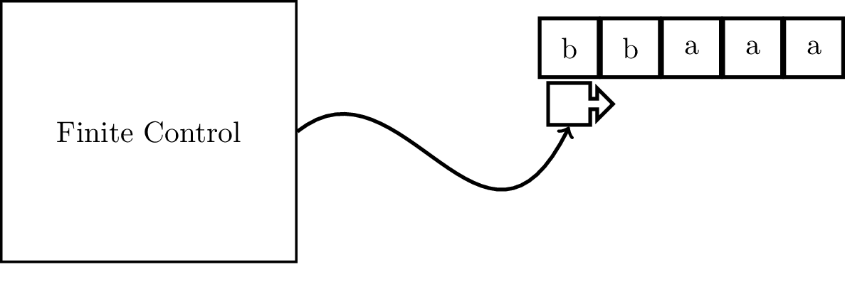
First, we'll introduce the idea of a "machine" as used in the theory of computation, which we'll be coming back to throughout the course. This idea originates from Turing in 1936, as what you may have heard of as a Turing machine. A machine has an input tape, divided into cells, with an input word written on it. The machine has a tape head that can scan the input tape, reading a symbol from each cell. The machine is also equipped with a finite set of instructions that will tell the machine how to act based on what it reads off of the tape. This set of instructions is encoded as a set of states.
The machine will read one tape cell, and therefore one symbol, at a time. Based on what it reads and the state that the machine is in, it will do the following:
What exactly does this model try to capture? What Turing attempted to do was formalize how computers worked, by which we mean the 1930s conception of what a computer is. In other words, he tried to formalize how human "computers" might "compute" a problem. We can view the finite state system as a set of instructions we might give to a person, that tells them what to do when they read a particular symbol. We allow this person to read and write on some paper and we let them have as much paper as they want.
Instead of jumping into working with the full model we described, we will start off by considering the most simplified model, where the machine can only read off of the tape (that is, it can't write) and it can only scan to the right—the tape head can never move to the left. This simplified model is what we call a finite automaton.
Since the machine only scans the input word to the right, it is guaranteed to stop when it reaches the end of the input string. Upon reading the entire input, the machine accepts or rejects the input word based on the state that the machine is in. This means that we can think of the machine as describing a set of strings—those that are accepted by the machine. This is the language of the machine and we can think of such a machine as computing the problem that its language corresponds to.
We call these finite automata because they have only a finite number of states. It wasn't stated explicitly, but based on the description, we also assume that the tape head can only move in one direction. Because of this restriction, it's not really necessary to think about the tape portion of the machine, at least for now.
We will give a formal definition for finite automata.
A deterministic finite automaton (DFA) is defined as a 5-tuple $A = (Q,\Sigma,\delta,q_0,F)$, where
Note that by our definition, $\delta$ must be defined for every state and input symbol. We call this a deterministic finite automaton because the transition function $\delta$ is uniquely determined by the state and input symbol.
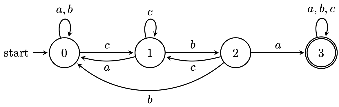
We can represent finite automata by drawing the important part of the machine: the state diagram. We draw each state as a circle and label it as appropriate. Transitions are represented as arrows, leaving one state and entering another, labelled by the appropriate input symbol. We denote accepting states by a double circle and we denote the start state by an arrow that comes in from nowhere in particular.
    \begin{tikzpicture}[shorten >=1pt,on grid,node distance=2.5cm,>=stealth,thick,auto]
        \node[state,initial] (0) {$0$};
        \node[state] (1) [right of=0]{$1$};
        \node[state] (2) [right of=1]{$2$};
        \node[state,accepting] (3) [right of=2]{$3$};
        \path[->]
            (0) edge [loop above] node {$a,b$} (0)
            (0) edge  node {$c$} (1)
            (1) edge [bend left=15] node {$a$} (0)
            (1) edge [loop above] node {$c$} (1)
            (1) edge  node {$b$} (2)
            (2) edge  node {$a$} (3)
            (3) edge [loop above] node {$a,b,c$} (3)
            (2) edge [bend left=15] node {$c$} (1)
            (2) edge [bend left=45] node {$b$} (0)
            ;
    \end{tikzpicture}
Suppose this DFA is $A = (Q, \Sigma, \delta, q_0, F)$. We can list all the parts that we've specified in our formal definition:
and $\delta$ is given by
| $a$ | $b$ | $c$ | |
|---|---|---|---|
| $0$ | $0$ | $0$ | $1$ |
| $1$ | $0$ | $2$ | $1$ |
| $2$ | $3$ | $0$ | $1$ |
| $3$ | $3$ | $3$ | $3$ |
    from automata.fa.dfa import DFA
    A = DFA(
        states=set('0123'),
        input_symbols=set('abc'),
        transitions={
            '0': {'a': '0', 'b': '0', 'c': '1'},
            '1': {'a': '0', 'b': '2', 'c': '1'},
            '2': {'a': '3', 'b': '0', 'c': '1'},
            '3': {'a': '3', 'b': '3', 'c': '3'}
        },
        initial_state='0',
        final_states={'3'}
    )
What does this machine do? We take a string and read it symbol by symbol and trace where we go based on the character. We see that strings that contain the substring $cba$ will end up in state 3, which is an accepting state, while those that don't never reach state 3. In other words, this machine determines whether a string over the alphabet $\{a,b,c\}$ contains the substring $cba$.
For example, suppose we want to run this machine on the string $bccbcbab$. We can view a computation on this machine by \[0 \xrightarrow{b} 0 \xrightarrow{c} 1 \xrightarrow{c} 1 \xrightarrow{b} 2 \xrightarrow{c} 1 \xrightarrow{b} 2 \xrightarrow{a} 3 \xrightarrow{b} 3.\] Since the machine is in state 3 upon completion of the string, $bccbcbab$ is accepted by the machine.
Now, we want to also formally define the notion of the set of words that our machine will accept. Intuitively, we have a sense of what acceptance and rejection means. We read a word and trace a path along the automaton and if we end up in an accepting state, the word is accepted and otherwise, the word is rejected.
First of all, it makes sense that we should be able to define this formally by thinking about the conditions that we've placed on the transition function. Since on each state $q$ and on each symbol $a$, we know exactly what state we end up on, it makes sense that each word takes us to a specific state.
So, we can extend the definition of the transition function so that it is a function from a state and a word to a state, $\delta^* : Q \times \Sigma^* \to Q$.
The function $\delta^* : Q \times \Sigma^* \to Q$ is defined by
It might be helpful to note that we can also approach this definition from the other direction. That is, instead of writing $w = ax$, we consider the factorization $w = xa$. Then the inductive part of our definition becomes $$\delta^*(q,xa) = \delta(\delta^*(q,x),a).$$ What's nice about using $w = xa$ is it naturally captures the idea that we often want to know what the "last step" of a computation is, while the $w = ax$ version focuses on the first step.
Another particularly nice property that we get out of this is the ability to split computations up by substring. The following is a nice induction exercise to prove on your own.
Let $A$ be a DFA $A = (Q, \Sigma, \delta, q_0, F)$. Then for all $u, v \in \Sigma^*$ and $q \in Q$, \[\delta^*(q,uv) = \delta^*(\delta^*(q,u),v).\]
Technically speaking, $\delta$ and $\delta^*$ are different functions, since one is a function on symbols and the other is a function on words. However, since $\delta^*$ is a natural extension of $\delta$, it's very easy to forget about the star and simply write $\delta$ for both functions. This is something I'm not too concerned about since the meaning is almost always clear.
A neat observation about $\delta^*$ is that if you are familiar with functional programming, then this is really just a fold or reduce on $\delta$. In other words, $\delta^*(q,w)$ would be something like (foldl δ q w).
Now, we can formally define the acceptance of a word by a DFA.
Let $A = (Q,\Sigma,\delta,q_0,F)$ be a DFA. We say $A$ accepts a word $w \in \Sigma^*$ when $\delta^*(q_0,w) \in F$. Then the language of a DFA $A$ is the set of all words accepted by $A$, $$L(A) = \{w \in \Sigma^* \mid \delta^*(q_0,w) \in F \}.$$ We also sometimes say that a word is recognized by $A$. We say that a language $L$ is accepted by a DFA $A$ if for all strings $w \in \Sigma^*$, $A$ accepts $w$ if $w \in L$ and $A$ rejects $w$ if $w \not \in L$. In other words, $L(A) = L$.
Now, we can begin to think about the kinds of problems that finite automata can solve. As a first example, we'll consider the idea of divisibility. Recall from discrete math that when we divide two integers, we don't always get another integer, which is nice because it spices things up a bit. However, we proved that we always get a unique quotient and remainder.
A constructive proof of the division theorem shows us how to do this, though we've likely employed such an algorithm numerous times throughout our schooling. This was noted by Blaise Pascal in the 1600s who showed that there's an algorithm for this in any base, not just decimal, and only by examining the sum of the digits of the number. This is based on the observation that remainders are essentially cyclic—we understand this structure to be $\mathbb Z_m$, the integers modulo $m$.
Let's consider the language $$ L_3 = \{w \in \{0,1\}^* \mid \text{$w$ is the binary representation of a number that is divisible by 3} \}.$$ In other words, this language describes the decision problem of whether a number is divisible by 3.
This is a fairly straightforward question to solve using a standard programming language, but notice that our model of computation places some fairly tight restrictions on what we can do: we can only remember a fixed amount of information and we must make a decision upon reading the string from left to right exactly once. This can be a bit of a challenge because we don't typically think of numerical problems from left to right—we usually begin from the right and go to the left.
The key here is that we need to be able to say something about the input we've read so far. If it's the end of the input, what kind of determination can we make about what we've read? If it's not the end of the input, what kind of information do we have that will allow us to update what we know, based on the next symbol that's read?
The other observation here is about the problem setting: how do we test for divisibility? A standard run through CS 141 will have you used to the idea of the modulus operator, which produces remainders. And a quick jaunt through discrete math will tell you that there are only ever a finite number of remainders and every number must have one. It seems like this is a viable option for the information we want to keep as states.