CMSC 28000 — Lecture 21

Computability

An interesting observation you may have noticed is that while $\{a^n \mid n \geq 0\}$ is accepted by a DFA, the language $\{a^n b^n \mid n \geq 0\}$ is not. And while a PDA can accept $\{a^n b^n \mid n \geq 0\}$, it can't accept $\{a^n b^n c^n \mid n \geq 0\}$. A natural question arises: can we play this game indefinitely? This is one of the things to keep in mind as we begin exploring the limits of computability. Generally speaking, computability theory is about whether a particular problem can be solved or not. Depending on what you've assumed about computers so far, this statement may or may not be obvious to you, but it's another thing to have it proved.

Computability theory is really the beginnings of the entire field of computer science and to see why, we need to go all the way back to the early 1900s. One of the central ideas in modern mathematical logic that came up at the time is distinguishing the notions of truth from proof. This might sound very abstract, but today, we would call these things the semantics and the synatx of a program, respectively.

The idea is that by separating the two, we can reduce proof and proof systems to mechanical manipulation of symbols. Recall that we use inference rules to describe valid steps in a proof. For instance, the rule \[\frac{\varphi \rightarrow \psi \quad \varphi}{\psi}\] says that if we know that $\varphi \rightarrow \psi$ and $\psi$, then we can conclude $\varphi$. It's common to think of this as saying something about the truth (that is, the semantics) of these statements, but it's actually saying something syntactic: if we see the strings $\varphi \rightarrow \psi$ and $\psi$ in our proof, we can add the string $\varphi$ to our proof.

This idea leads to a few questions.

Do the syntactic rules of proof systems coincide with the semantic values that we assign to logical formulas?
Since proof systems are syntactic, is is possible to find an algorithm that can mechanically construct a proof and determine the validity of a given statement?

The first question was answered by Kurt Gödel by the Completeness Theorem in 1929. The second question was posed by Hilbert in 1928, as the Entscheidungsproblem.

In essence, this second question is about computation and it is what kicked off a flurry of activity in the 1930s trying to nail down what exactly it means to compute something. Gödel used what are called $\mu$-recursive functions to try to do this. Alonzo Church defined the $\lambda$-calculus for this purpose. Emil Post defined what are called Post systems, which are a kind of string rewriting system.

And in 1936, Alan Turing defined what we now call Turing machines.

Turing machines

First, we'll try to understand what a Turing machine is informally. Remember that we started out with the finite automaton, considered the simplest model of computation. This is just some finite set of states, or memory, and some transitions. We can do a lot of useful things with FAs but there are many languages that FAs aren't powerful enough to recognize, such as $a^n b^n$. However, we can enhance the power of the machine by adding a stack. This gives us the ability to recognize a larger class of languages.

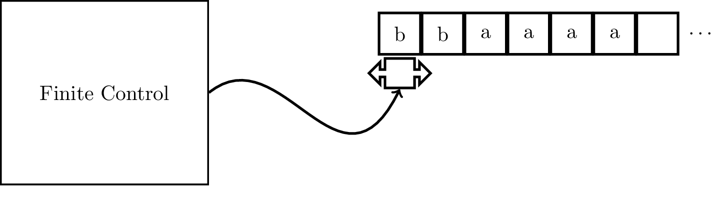
We can think of a Turing machine in the same way. A Turing machine is just a finite automaton with the two main restrictions we placed on it now lifted. That is, the tape that we placed our input on before which was read-only can now be written, and our tape is infinitely long. Furthermore, we can move however we like on the tape, unlike the pushdown stack.

A Turing machine is a 7-tuple $M = (Q,\Sigma,\Gamma,\delta,q_0,q_{\mathsf{acc}},q_{\mathsf{rej}})$, where

$Q$ is a finite set of states,
$\Sigma$ is a finite input alphabet that does not contain the blank symbol $\Box$,
$\Gamma$ is a finite tape alphabet with a blank symbol $\Box \in \Gamma$ and $\Sigma \subseteq \Gamma$,
$\delta: Q \times \Gamma \to Q \times \Gamma \times \{\leftarrow,\rightarrow\}$ is the transition function,
$q_0 \in Q$ is the initial state,
$q_{\mathsf{acc}} \in Q$ is the accepting state,
$q_{\mathsf{rej}} \in Q$ is the rejecting state, with $q_{\mathsf{acc}} \neq q_{\mathsf{rej}}$.

In our model, we have a one-sided infinitely long tape, with the machine starting its computation with the input on the tape beginning at the left end of the tape. The input string is followed by infinitely many blank symbols $\Box$ at the right. The transition function is deterministic.

What exactly does this model try to capture? What Turing attempted to do was formalize how computers worked, by which we mean the 1930s conception of what a computer is. In other words, he tried to formalize how human "computers" might "compute" a problem. We can view the finite state system as a set of instructions we might give to a person, that tells them what to do when they read a particular symbol. We allow this person to read and write on some paper and we let them have as much paper as they want.

In the course of a computation on a Turing machine, one of three outcomes will occur.

The machine enters the accepting state and accepts and halts.
The machine enters the rejecting state and rejects and halts.
The machine never enters the accepting or rejecting state and does not halt.

For a Turing machine $M$ and an input word $w$, if the computation of $M$ on $w$ enters the accepting state, then we say that $M$ accepts $w$. Likewise, if the computation of $M$ on $w$ enters the rejecting state, then we say $M$ rejects $w$. We call the set of strings that are accepted by $M$ the language of $M$, denoted $L(M)$.

It is important to note that in these definitions, $w$ is the string that the computation begins with, not the string that is on the tape when the computation halts.

Notice that since we now have three possibilities, we have more notions of what it means for a Turing amchine to accept a language.

A Turing machine $M$ recognizes a language $L$ if every word in $L$ is accepted by $M$ and for every input not in $L$, $M$ either rejects the word or does not halt. A language $L$ is recognizable if some Turing machine recognizes it.

A Turing machine $M$ decides a language $L$ if every word in $L$ is accepted by $M$ and every input not in $L$ is rejected by $M$. A language $L$ is decidable if some Turing machine decides it.

These notions lead directly to two classes of languages.

The class of (Turing-)recognizable languages is the class of languages that can be recognized by a Turing machine. This class is also called the class of recursively enumerable languages.

The class of (Turing-)decidable languages is the class of languages that can be decided by a Turing machine. This class is also called the class of recursive languages.

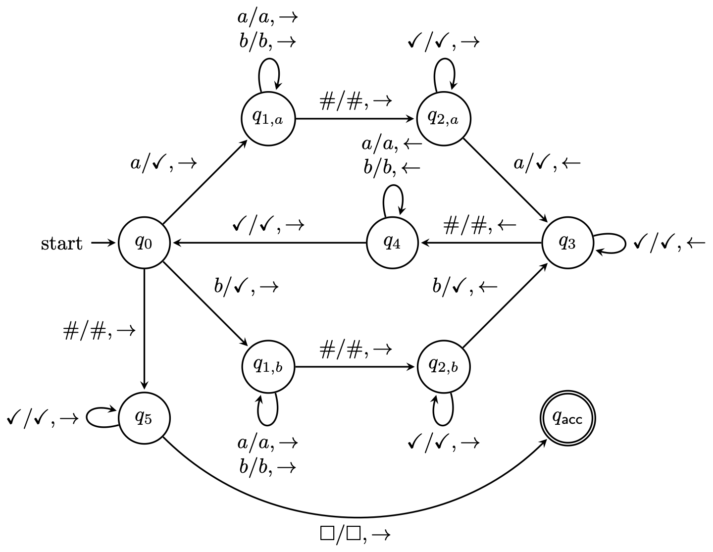
Consider the language $L = \{ x \# x \mid x \in \{a,b\}^* \}$. This is the language where we have two copies of the same word divided by $\#$ over the alphabet $\{a,b\}$. It is not hard to show that this language is not context-free. How would we build a Turing machine for this? We can think of what we'd like such a machine to do at a high level.

Read a symbol and remember what it is. Mark the cell.
Go to the right of the $\#$ to the first unmarked symbol. If there is no $\#$, then reject.
Check to see if the symbol is the same one that we just marked. If the symbols are not the same, reject.
Mark the cell.
Go to the left past the $\#$ and until a marked cell is encountered.
Go to the symbol to the right.
If the current symbol is unmarked, repeat the process from Step 1. If the current symbol is $\#$, go to the next step.
Scan to the right. If an unmarked symbol is encountered, reject. If a blank symbol is encountered, accept.

As always, the challenge is formalizing this mechanically. We will attempt this and see why we will not do this anymore. Here is the formal description. Let $M = (Q, \Sigma, \Gamma, \delta, q_0, q_{\mathsf{acc}}, q_{\mathsf{rej}})$ where

$Q = \{q_0, q_{1,a}, q_{1,b}, q_{2,a}, q_{2,b}, q_3, q_4, q_5, q_{\mathsf{acc}}, q_{\mathsf{rej}}\}$
$\Sigma = \{a,b,\#\}$,
$\Gamma = \{a,b, \#, \Box, \checkmark\}$,

and the transition function $\delta$ is defined

	$a$	$b$	$\#$	$\Box$	$\checkmark$
$q_0$	$(q_{1,a}, \checkmark, \rightarrow)$	$(q_{1,b}, \checkmark, \rightarrow)$	$(q_5, \#, \rightarrow)$	reject	reject
$q_{1,a}$	$(q_{1,a}, a, \rightarrow)$	$(q_{1,a}, b, \rightarrow)$	$(q_{2,a}, \#, \rightarrow)$	reject	reject
$q_{1,b}$	$(q_{1,b}, a, \rightarrow)$	$(q_{1,b}, b, \rightarrow)$	$(q_{2,b}, \#, \rightarrow)$	reject	reject
$q_{2,a}$	$(q_3, \checkmark, \leftarrow)$	reject	reject	reject	$(q_{2,a}, \checkmark, \rightarrow)$
$q_{2,b}$	reject	$(q_3, \checkmark, \leftarrow)$	reject	reject	$(q_{2,b}, \checkmark, \rightarrow)$
$q_3$	reject	reject	$(q_4, \#, \leftarrow)$	reject	$(q_3, \checkmark, \leftarrow)$
$q_4$	$(q_4, a, \leftarrow)$	$(q_4, b, \leftarrow)$	reject	reject	$(q_0, \checkmark, \rightarrow)$
$q_5$	reject	reject	reject	$(q_{\mathsf{acc}}, \Box, \rightarrow)$	$(q_5, \checkmark, \rightarrow)$

Here, "reject" is shorthand for the transition $(q_{\mathsf{rej}}, \sigma, \rightarrow)$ for whichever $\sigma \in \Gamma$ was read to make it more clear to the reader which transitions reject (otherwise, it gets lost in the table).

Notice that we use $\checkmark$ as our "mark". This belongs on the tape alphabet, since we never want to see an input string that uses $\checkmark$.

Here is the state diagram. Note that the rejecting state and its incoming transitions are not shown.


\begin{tikzpicture}[shorten >=1pt,on grid,node distance=3cm,>=stealth,thick,auto]
    \node[state,initial] (0) []{$q_0$};
    \node[state] (1a) [above right of=0]{$q_{1,a}$};
    \node[state] (1b) [below right of=0]{$q_{1,b}$};
    \node[state] (2a) [right of=1a]{$q_{2,a}$};
    \node[state] (2b) [right of=1b]{$q_{2,b}$};
    \node[state] (3) [below right of=2a]{$q_3$};
    \node[state] (4) [left of=3]{$q_4$};
    \node[state] (5) [below of=0]{$q_5$};
    \node[state,accepting] (a) [below of=3]{$q_{\mathsf{acc}}$};
    \path[->]
        (0) edge  node {$a/\checkmark, \rightarrow$} (1a)
        (0) edge  node {$b/\checkmark, \rightarrow$} (1b)
        (0) edge [left] node {$\#/\#, \rightarrow$} (5)
        (1a) edge [loop above] node [align=center] {$a/a, \rightarrow$ \\ $b/b, \rightarrow$} (1a)
        (1a) edge  node {$\#/\#, \rightarrow$} (2a)
        (1b) edge [loop below] node[align=center]  {$a/a, \rightarrow$ \\ $b/b, \rightarrow$} (1b)
        (1b) edge  node {$\#/\#, \rightarrow$} (2b)
        (2a) edge [loop above] node {$\checkmark/\checkmark, \rightarrow$} (2a)
        (2b) edge [loop below] node {$\checkmark/\checkmark, \rightarrow$} (2b)
        (2a) edge  node {$a/\checkmark, \leftarrow$} (3)
        (2b) edge  node {$b/\checkmark, \leftarrow$} (3)
        (3) edge [loop right] node {$\checkmark/\checkmark, \leftarrow$} (3)
        (3) edge [above] node {$\#/\#, \leftarrow$} (4)
        (4) edge [loop above] node [align=center] {$a/a, \leftarrow$ \\ $b/b,\leftarrow$} (4)
        (4) edge [above] node {$\checkmark/\checkmark, \rightarrow$} (0)
        (5) edge [loop left] node {$\checkmark/\checkmark, \rightarrow$} (5)
        (5) edge [below,bend right=45] node {$\Box/\Box, \rightarrow$} (a)
        ;
\end{tikzpicture}

Here's some runnable code.


from automata.tm.dtm import DTM
A = DTM(
    states={'0', '1a', '1b', '2a', '2b', '3', '4', '5', 'accept'},
    input_symbols=set('ab#'),
    tape_symbols=set('ab#X.'),
    transitions={
        '0': {
            'a': ('1a', 'X', 'R'),
            'b': ('1b', 'X', 'R'),
            '#': ('5', '#', 'R'),
        },
        '1a': {
            'a': ('1a', 'a', 'R'),
            'b': ('1a', 'b', 'R'),
            '#': ('2a', '#', 'R'),
        },
        '1b': {
            'a': ('1b', 'a', 'R'),
            'b': ('1b', 'b', 'R'),
            '#': ('2b', '#', 'R'),
        },
        '2a': {
            'a': ('3', 'X', 'L'),
            'X': ('2a', 'X', 'R'),
        },
        '2b': {
            'b': ('3', 'X', 'L'),
            'X': ('2b', 'X', 'R'),
        },
        '3': {
            '#': ('4', '#', 'L'),
            'X': ('3', 'X', 'L'),
        },
        '4': {
            'a': ('4', 'a', 'L'),
            'b': ('4', 'b', 'L'),
            'X': ('0', 'X', 'R'),
        },
        '5': {
            '.': ('accept', '.', 'R'),
            'X': ('5', 'X', 'R'),
        },
    },
    initial_state='0',
    blank_symbol='.',
    final_states={'accept'}
)


>>> for x in A.read_input_stepwise('abb#abb'):
...     print(x)
... 
TMConfiguration('0', TMTape('abb#abb', '.', 0))
TMConfiguration('1a', TMTape('Xbb#abb', '.', 1))
TMConfiguration('1a', TMTape('Xbb#abb', '.', 2))
TMConfiguration('1a', TMTape('Xbb#abb', '.', 3))
TMConfiguration('2a', TMTape('Xbb#abb', '.', 4))
TMConfiguration('3', TMTape('Xbb#Xbb', '.', 3))
TMConfiguration('4', TMTape('Xbb#Xbb', '.', 2))
TMConfiguration('4', TMTape('Xbb#Xbb', '.', 1))
TMConfiguration('4', TMTape('Xbb#Xbb', '.', 0))
TMConfiguration('0', TMTape('Xbb#Xbb', '.', 1))
TMConfiguration('1b', TMTape('XXb#Xbb', '.', 2))
TMConfiguration('1b', TMTape('XXb#Xbb', '.', 3))
TMConfiguration('2b', TMTape('XXb#Xbb', '.', 4))
TMConfiguration('2b', TMTape('XXb#Xbb', '.', 5))
TMConfiguration('3', TMTape('XXb#XXb', '.', 4))
TMConfiguration('3', TMTape('XXb#XXb', '.', 3))
TMConfiguration('4', TMTape('XXb#XXb', '.', 2))
TMConfiguration('4', TMTape('XXb#XXb', '.', 1))
TMConfiguration('0', TMTape('XXb#XXb', '.', 2))
TMConfiguration('1b', TMTape('XXX#XXb', '.', 3))
TMConfiguration('2b', TMTape('XXX#XXb', '.', 4))
TMConfiguration('2b', TMTape('XXX#XXb', '.', 5))
TMConfiguration('2b', TMTape('XXX#XXb', '.', 6))
TMConfiguration('3', TMTape('XXX#XXX', '.', 5))
TMConfiguration('3', TMTape('XXX#XXX', '.', 4))
TMConfiguration('3', TMTape('XXX#XXX', '.', 3))
TMConfiguration('4', TMTape('XXX#XXX', '.', 2))
TMConfiguration('0', TMTape('XXX#XXX', '.', 3))
TMConfiguration('5', TMTape('XXX#XXX', '.', 4))
TMConfiguration('5', TMTape('XXX#XXX', '.', 5))
TMConfiguration('5', TMTape('XXX#XXX', '.', 6))
TMConfiguration('5', TMTape('XXX#XXX.', '.', 7))
TMConfiguration('accept', TMTape('XXX#XXX..', '.', 8))

As with the PDA, we see that there is a notion of a configuration for a Turing machine. That is, we need a way to talk about the "current state" of the machine as it's carrying out its computation. We can imagine this like a PDA, as a tuple containing the current state, tape contents, and location of the tape head. Howeer, there is a slightly more clever and convenient scheme we can use.

A configuration of a Turing machine $M = (Q, \Sigma, \Gamma, \delta, q_0, q_{\mathsf{acc}}, q_{\mathsf{rej}})$ is a string $uqv$, where

$q \in Q$ is the current state,
the current tape contents is $uv$, where $u,v \in \Gamma^*$, and
the tape head is located on top of the tape cell corresponding to the first symbol of $v$.

The initial configuration of $M$ when run on input word $w$ is the string $q_0 w$. An accepting configuration of $M$ is a string $u q_{\mathsf{acc}} v$ with $u,v \in \Gamma^*$. Similarly, a rejecting configuration of $M$ is a string $u q_{\mathsf{rej}} v$ with $u,v \in \Gamma^*$.

Unlike with PDAs, we don't need a separate notion of the input to be consumed because that information is on the tape and can be changed during the course of computation.

Notice that the only requirement for an accepting (respectively, rejecting) configuration is the presence of the state $q_{\mathsf{acc}}$ ($q_{\mathsf{rej}}$) in the configuration and it doesn't matter what else is on the tape.

Suppose our Turing machine is in state $q_5$ and the contents of the tape and the position of the tape head are as below.

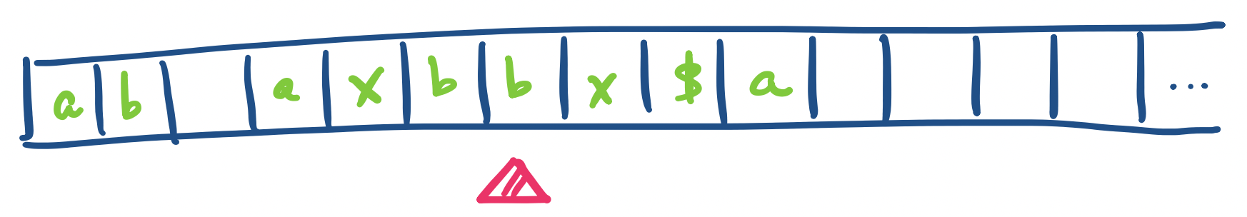
Then the configuration would be $ab \Box axbq_5bx\$a$. Notice that we explicitly denote blank cells when there are non-blank cells before and after, but we do not include the infinitely many blank cells to the right of the rightmost non-blank cell.

An underappreciated aspect of configurations is that they are really just strings. This means that with a sufficiently powerful string rewriting system, one can encode the transitions of a Turing machine as the rules of a rewriting system and have the rewriting system simulate a computation on the Turing machine.

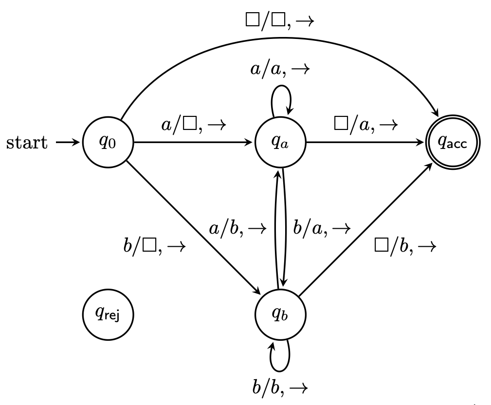
Because Turing machines are able to modify the contents of the tape, we often use high level descriptions like "copy the contents of the tape" or "shift the contents to the right". But can we really do those things? Let's see a simple example of one such subroutine—shifting the contents of a tape one cell to the right.

The idea is to write a blank in the tape cell that we start in while remembering the symbol that we overwrote in the state memory. When we move to the right, we write down the last symbol we saw and remember the symbol that we overwrote and repeat this process until we see a blank cell.

We'll define the machine $M = (Q, \Sigma, \Gamma, \delta, q_0, q_{\mathsf{acc}}, q_{\mathsf{rej}})$ that will shift things over by one cell by

$Q = \{q_0, q_{\mathsf{acc}}, q_{\mathsf{rej}}\} \cup \{q_a \mid a \in \Sigma\}$
$\Gamma = \Sigma \cup \{\Box\}$

and the transition function $\delta$ is defined by

$\delta(q_0, a) = (q_a, \Box, \rightarrow)$ for $a \in \Sigma$,
$\delta(q_0, \Box) = (q_{\mathsf{acc}}, \Box, \rightarrow)$,
$\delta(q_b, a) = (q_a, b, \rightarrow)$ for $a,b \in \Sigma$,
$\delta(q_a, \Box) = (q_{\mathsf{acc}}, a, \rightarrow)$ for $a \in \Sigma$.

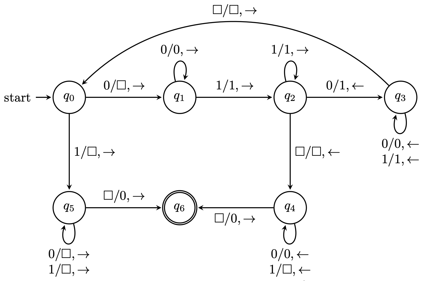
Here is the state diagram for the "shift over" machine for $\Sigma = \{a,b\}$.


\begin{tikzpicture}[shorten >=1pt,on grid,node distance=3cm,>=stealth,thick,auto]
    \node[state,initial] (0) []{$q_0$};
    \node[state] (a) [right of=0]{$q_{a}$};
    \node[state] (b) [below of=a]{$q_{b}$};
    \node[state,accepting] (acc) [right of=a]{$q_{\mathsf{acc}}$};
    \node[state] (rej) [left of=b]{$q_{\mathsf{rej}}$};
    \path[->]
        (0) edge  node {$a/\Box, \rightarrow$} (a)
        (0) edge [below left] node {$b/\Box, \rightarrow$} (b)
        (0) edge [bend left=60] node {$\Box/\Box, \rightarrow$} (acc)
        (a) edge  node {$\Box/a, \rightarrow$} (acc)
        (b) edge [below right] node {$\Box/b, \rightarrow$} (acc)
        (a) edge [bend left=5] node {$b/a, \rightarrow$} (b)
        (b) edge [bend left=5] node {$a/b, \rightarrow$} (a)
        (a) edge [loop above] node {$a/a, \rightarrow$} (a)
        (b) edge [loop below] node {$b/b, \rightarrow$} (b)
        ;
\end{tikzpicture}

Notice that no transitions go to the rejecting state.

So now that we've shifted the tape contents to the right, we can return to the cell that we started in by searching for a blank cell—the one that we inserted when we first began the shifting process.


from automata.tm.dtm import DTM
A = DTM(
    states={'0', 'a', 'b', 'accept'},
    input_symbols=set('ab'),
    tape_symbols=set('ab.'),
    transitions={
        '0': {
            '.': ('accept', '.', 'R'),
            'a': ('a', '.', 'R'),
            'b': ('b', '.', 'R')
        },
        'a': {
            '.': ('accept', 'a', 'R'),
            'a': ('a', 'a', 'R'),
            'b': ('b', 'a', 'R')
        },
        'b': {
            '.': ('accept', 'b', 'R'),
            'a': ('a', 'b', 'R'),
            'b': ('b', 'b', 'R')
        },
    },
    initial_state='0',
    blank_symbol='.',
    final_states={'accept'}
)


>>> list(A.read_input_stepwise('ababb'))
[TMConfiguration('0', TMTape('ababb', '.', 0)),
 TMConfiguration('a', TMTape('.babb', '.', 1)),
 TMConfiguration('b', TMTape('.aabb', '.', 2)),
 TMConfiguration('a', TMTape('.abbb', '.', 3)),
 TMConfiguration('b', TMTape('.abab', '.', 4)),
 TMConfiguration('b', TMTape('.abab.', '.', 5)),
 TMConfiguration('accept', TMTape('.ababb.', '.', 6))]

It's this usage of the Turing machine that opens the model to computation beyond decision problems. If we consider the contents left on the tape of a Turing machine after it halts to be the "output" of the Turing machine, then we can think of a Turing machine as "computing" some function that, when given some input $w$, produces some output.

Recall the monus function, which, when given two natural numbers $m$ and $n$, we have \[m \dotdiv n = \begin{cases} 0 & \text{if $m \lt n$,} \\ m-n & \text{if $m \geq n$.} \end{cases}\] Here, we define a Turing machine that on input $0^m 1 0^n$, halts with $0^{m \dotdiv n}$ left on the tape.


from automata.tm.dtm import DTM
A = DTM(
    states=set(range(7)),
    input_symbols='01',
    tape_symbols='01.',
    transitions={
        0: {
            '0': (1, '.', 'R'),
            '1': (5, '.', 'R'),
        },
        1: {
            '0': (1, '0', 'R'),
            '1': (2, '1', 'R')
        },
        2: {
            '0': (3, '1', 'L'),
            '1': (2, '1', 'R'),
            '.': (4, '.', 'L')
        },
        3: {
            '0': (3, '0', 'L'),
            '1': (3, '1', 'L'),
            '.': (0, '.', 'R')
        },
        4: {
            '0': (4, '0', 'L'),
            '1': (4, '.', 'L'),
            '.': (6, '0', 'R')
        },
        5: {
            '0': (5, '.', 'R'),
            '1': (5, '.', 'R'),
            '.': (6, '.', 'R'),
        },
    },
    initial_state=0,
    blank_symbol='.',
    final_states={6}
)


>>> for x in A.read_input_stepwise('0000001000'):
...     print(x)
... 
TMConfiguration(0, TMTape('0000001000', '.', 0))
TMConfiguration(1, TMTape('.000001000', '.', 1))
TMConfiguration(1, TMTape('.000001000', '.', 2))
TMConfiguration(1, TMTape('.000001000', '.', 3))
TMConfiguration(1, TMTape('.000001000', '.', 4))
TMConfiguration(1, TMTape('.000001000', '.', 5))
TMConfiguration(1, TMTape('.000001000', '.', 6))
TMConfiguration(2, TMTape('.000001000', '.', 7))
TMConfiguration(3, TMTape('.000001100', '.', 6))
TMConfiguration(3, TMTape('.000001100', '.', 5))
TMConfiguration(3, TMTape('.000001100', '.', 4))
TMConfiguration(3, TMTape('.000001100', '.', 3))
TMConfiguration(3, TMTape('.000001100', '.', 2))
TMConfiguration(3, TMTape('.000001100', '.', 1))
TMConfiguration(3, TMTape('.000001100', '.', 0))
TMConfiguration(0, TMTape('.000001100', '.', 1))
TMConfiguration(1, TMTape('..00001100', '.', 2))
TMConfiguration(1, TMTape('..00001100', '.', 3))
TMConfiguration(1, TMTape('..00001100', '.', 4))
TMConfiguration(1, TMTape('..00001100', '.', 5))
TMConfiguration(1, TMTape('..00001100', '.', 6))
TMConfiguration(2, TMTape('..00001100', '.', 7))
TMConfiguration(2, TMTape('..00001100', '.', 8))
TMConfiguration(3, TMTape('..00001110', '.', 7))
TMConfiguration(3, TMTape('..00001110', '.', 6))
TMConfiguration(3, TMTape('..00001110', '.', 5))
TMConfiguration(3, TMTape('..00001110', '.', 4))
TMConfiguration(3, TMTape('..00001110', '.', 3))
TMConfiguration(3, TMTape('..00001110', '.', 2))
TMConfiguration(3, TMTape('..00001110', '.', 1))
TMConfiguration(0, TMTape('..00001110', '.', 2))
TMConfiguration(1, TMTape('...0001110', '.', 3))
TMConfiguration(1, TMTape('...0001110', '.', 4))
TMConfiguration(1, TMTape('...0001110', '.', 5))
TMConfiguration(1, TMTape('...0001110', '.', 6))
TMConfiguration(2, TMTape('...0001110', '.', 7))
TMConfiguration(2, TMTape('...0001110', '.', 8))
TMConfiguration(2, TMTape('...0001110', '.', 9))
TMConfiguration(3, TMTape('...0001111', '.', 8))
TMConfiguration(3, TMTape('...0001111', '.', 7))
TMConfiguration(3, TMTape('...0001111', '.', 6))
TMConfiguration(3, TMTape('...0001111', '.', 5))
TMConfiguration(3, TMTape('...0001111', '.', 4))
TMConfiguration(3, TMTape('...0001111', '.', 3))
TMConfiguration(3, TMTape('...0001111', '.', 2))
TMConfiguration(0, TMTape('...0001111', '.', 3))
TMConfiguration(1, TMTape('....001111', '.', 4))
TMConfiguration(1, TMTape('....001111', '.', 5))
TMConfiguration(1, TMTape('....001111', '.', 6))
TMConfiguration(2, TMTape('....001111', '.', 7))
TMConfiguration(2, TMTape('....001111', '.', 8))
TMConfiguration(2, TMTape('....001111', '.', 9))
TMConfiguration(2, TMTape('....001111.', '.', 10))
TMConfiguration(4, TMTape('....001111.', '.', 9))
TMConfiguration(4, TMTape('....00111..', '.', 8))
TMConfiguration(4, TMTape('....0011...', '.', 7))
TMConfiguration(4, TMTape('....001....', '.', 6))
TMConfiguration(4, TMTape('....00.....', '.', 5))
TMConfiguration(4, TMTape('....00.....', '.', 4))
TMConfiguration(4, TMTape('....00.....', '.', 3))
TMConfiguration(6, TMTape('...000.....', '.', 4))

This notion of a Turing machine computing a function can be used to define the following class of functions.

A function $f: \Sigma^* \to \Sigma^*$ is a computable function if there exists a Turing machine $M$ that on every input $w \in \Sigma^*$ halts with only $f(w)$ left on its tape.