It's worth thinking about what happens if we try the same thing that we've done with our previous machines and make some modifications to Turing machines. For instance, if we remember the finite automaton, we have the deterministic and nondeterministic variants. As it turned out, the power of the machines were exactly the same, in that they both recognized exactly the same class of languages. However, there was a tradeoff in the number of states between the two models. Similarly, we recall that this same variation yields vastly different results for the pushdown automaton. The deterministic pushdown automata could recognize fewer languages that could be recognized by the nondeterministic machine.
We now explore the same kinds of ideas with Turing machines. The goal is to show that the Turing machine is actually fairly powerful and to give us some tools when working with them.
As with PDAs, it is helpful to define a notion of the current state of the machine, or the configuration. For Turing machines we need to know the following pieces of information:
A configuration of a Turing machine $M = (Q, \Sigma, \Gamma, \delta, q_0, q_{\mathsf{acc}}, q_{\mathsf{rej}})$ is a string $uqv$, where
The initial configuration of $M$ when run on input word $w$ is the string $q_0 w$. An accepting configuration of $M$ is a string $u q_{\mathsf{acc}} v$ with $u,v \in \Gamma^*$. Similarly, a rejecting configuration of $M$ is a string $u q_{\mathsf{rej}} v$ with $u,v \in \Gamma^*$.
Unlike with PDAs, we don't need a separate notion of the input to be consumed because that information is on the tape and can be changed during the course of computation.
Notice that the only requirement for an accepting (respectively, rejecting) configuration is the presence of the state $q_{\mathsf{acc}}$ ($q_{\mathsf{rej}}$) in the configuration and it doesn't matter what else is on the tape.
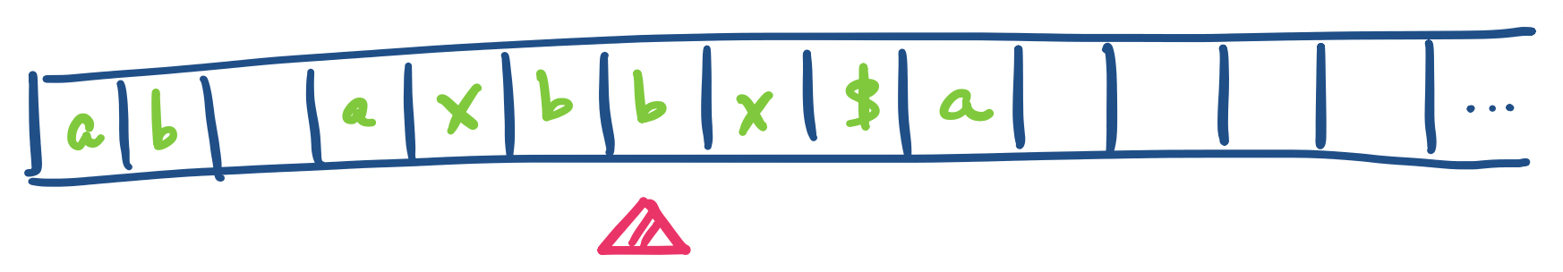
Suppose our Turing machine is in state $q_5$ and the contents of the tape and the position of the tape head are as below.
Then the configuration would be $ab \Box axbq_5bx\$a$. Notice that we explicitly denote blank cells when there are non-blank cells before and after, but we do not include the infinitely many blank cells to the right of the rightmost non-blank cell.
An underappreciated aspect of configurations is that they are really just strings. This means that with a sufficiently powerful string rewriting system, one can encode the transitions of a Turing machine as the rules of a rewriting system and have the rewriting system simulate a computation on the Turing machine.
One example of how we can modify the Turing machine model is to ask what if instead of using only a single tape, we allowed the Turing machine to have multiple tapes with tape heads that move independently of each other? That is, for $k$ tapes, we modify the definition so we have the transition function $\delta : Q \times \Gamma^k \to Q \times \Gamma^k \times \{L,R\}^k$.
Every language recognized by a multi-tape Turing machine can be recognized by a single tape Turing machine.
We show how to simulate a multi-tape Turing machine on a single-tape Turing machine. The idea is to store all the contents of each tape on the single tape and separate each tape as required. We also keep track of the tape head positions on each of the virtual tapes.
What does this machine look like? We describe a Turing machine which simulates a $k$-tape TM $M$ as follows:
Since a single-tape Turing machine can obviously be simulated by a $k$-tape Turing machine, this tells us that the two models are equivalent.
Our current Turing machine is defined to be deterministic. However, we can show that we can introduce nondeterminism without increasing or decreasing the power of the model.
In a nondeterministic Turing machine, the transition function is a function $\delta: Q \times \Gamma \to 2^{Q \times \Gamma \times \{L,R\}}$. That is, our transition function maps onto a set of possible transitions.
As with other nondeterministic models, we can view the computation of a nondeterministic Turing machine as a tree, where each branch represents a possible choice or guess. Then a nondeterministic Turing machine accepts a word if at least one branch of the computation tree enters an accepting state. It's important to note that, as with other nondeterministic models, a nondeterministic Turing machine $M$ on an input string $w$
Every nondeterministic Turing machine has an equivalent deterministic Turing machine.
The idea behind this proof is to construct a Turing machine that performs a breadth-first search of the computation tree. Recall that the transition function of a nondeterministic Turing machine is a function $\delta: Q \times \Gamma \to 2^{Q \times \Gamma \times \{\leftarrow, \rightarrow\}}$. Since $Q$ and $\Gamma$ are both finite, any single transition has a finite number of choices, so every node in the tree is guaranteed to have finitely many children.
Since we do a breadth-first search, if the machine accepts the input string, the branch containing an accepting configuration will be finite and we will eventually find it. Similarly, if the machine rejects the input string, we will eventually find all rejecting configurations. And if the machine runs forever, then the search will continue forever.
We use a 3-tape deterministic machine to simulate the nondeterministic machine $N$. We can do this because we have just conveniently showed that a $k$-tape machine is equivalent to a single tape machine. The tapes are used as follows:
The third tape is what will allow us to navigate through the tree. Let $k = \max\limits_{q \in Q, a \in \Gamma} |\delta(q,a)|$. For each node, we assign a value to each child from $1$ to $k$. Then by considering a string over the alphabet $\{1,\dots,k\}$, we follow a particular branch at each set of choices, starting from the root of the tree.

Note that not every string over $\{1,\dots,k\}$ will correspond to a valid address, since not every nondeterministic set of choices is guaranteed to have as many as $k$ choices. But this is fine, since that address simply will not correspond to a node. Then by enumerating through every string, we are guaranteed to reach every node of the computation tree.
Now, the machine operates as follows:
This gives us the following corollary.
A language is recognizable if and only if some nondeterministic Turing machine recognizes it.
However, if we know that a nondeterministic Turing machine will always halt on every branch of its computation, then the corresponding deterministic machine will be also always halt. This leads to the following result.
A language is decidable if and only if some nondeterministic Turing machine decides it.
Something you might notice or object to is that simulating a nondeterministic Turing machine with a deterministic machine can potentially take a very long time. Since we're performing a breadth-first search, this means that we're looking at a computation that's exponential in the length of the shortest accepting path in the nondeterministic computation tree. But that's okay, because we only care whether our deterministic machine is able to recognize or decide any language that a nondeterministic machine is capable of recognizing.
But for argument's sake, let's suppose that we do care about the time that it takes. We can measure this: how many steps is the computation on our machine? We can apply our notions of efficiency from other CS courses and consider polynomially many steps to be good or efficient. So suppose that I have a nondeterministic TM that has an accepting computation branch that's polynomially long in the size of the input. Is it possible to simulate or come up with a way to solve the same problem deterministically, but still end up with only a polynomially long computation?
The answer is: we don't know! Because this question is exactly the P vs. NP problem.