Implementing Kruskal's algorithm
Again, we are faced with the question of how to efficiently implement an algorithm and again, we will be making use of a fancy data structure.
Here, we are faced with a bit of a different problem than we encountered with Dijkstra's or Prim's algorithms. Instead of maintaining a set of explored vertices, we need to keep track of multiple sets and manipulate these sets. Looking back at the algorithm, we have three things we need to be able to do:
- create new sets,
- figure out which set an element belongs to,
- take the union of two sets.
One important property that we can take advantage of is the fact that these sets are going to be disjoint. This is helpful, because we know that an element can only belong to exactly one set.
The problem of managing multiple disjoint sets with these operations turns out to be a problem of its own, called the Union-Find problem, first studied by Galler and Fisher in 1964. This problem is closely related to what we're doing with Kruskal's algorithm, which is managing multiple connected components of a graph.
Ultimately, to solve this problem, we need a data structure to represent disjoint sets. Such a data structure has the following operations:
make-set(v): make a new set from an element $v$,
find-set(v): find which set a given element $v$ is in,
union(u,v): take the union of the two sets containing $u$ and $v$.
Spookily, these correspond exactly to our operations above.
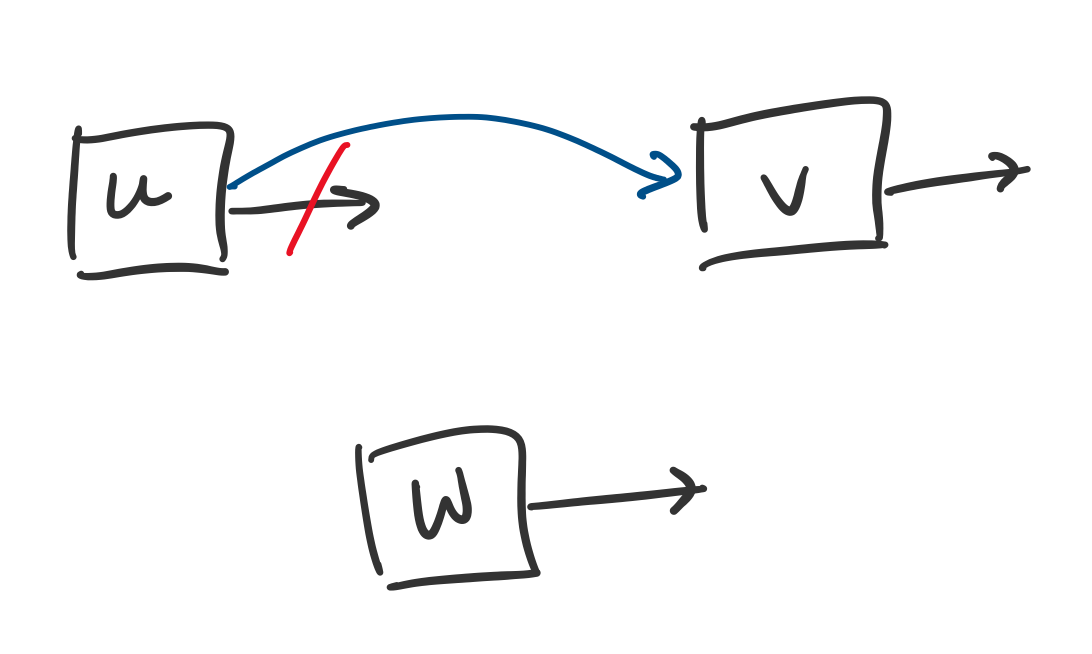
One question is how to "find" a set. Typically, we distinguish sets by choosing a "representative" of the set. So if $u$ and $v$ are in the same set and $u$ is the representative for that set, then find-set(u) and find-set(v) will both return $u$.
Here is a simple (but not optimal) implementation of this data structure: use linked lists to keep track of these sets and maintain pointers to each element. The nodes for each element will contain the element and a pointer to another element that belongs to the same set. If the node contains a null pointer, then it is the representative for that set.
Based on this description, it is easy to see that make-set can be performed in $O(1)$ time: just make a list with a single node. It is also not too hard to see how to perform a union: just link the representative of a set to the representative of another set. In principle, this requires $O(1)$ time, since we just change a pointer, but this assumes that we have located the representatives of both sets.
This question is linked to the remaining operation: find. One realizes that if we apply unions arbitrarily, we can end up with situations where find can require $O(n)$ time. One way to deal with this is to enforce a priority on which element becomes the representative of a set. One can show that by making the representative of the larger of the two sets the new representative for the union of the two sets, we can guarantee that find has a running time of $O(\log n)$. This is accomplished by storing an additional piece of information, the size of the set.
This gives us the following running times for our operations:
make-set(v) in $O(1)$ time
find-set(v) in $O(\log n)$ time
union(u,v) in $O(1)$ time.
Now, we can return to analyzing Kruskal's algorithm. Luckily, we don't really need to rewrite our algorithm since the Union-Find data structure uses the same operations we've used in the algorithm above.
Kruskal's algorithm has running time $O(m \log n)$, where $m = |E|$ and $n = |V|$.
First, we sort the edges by weight, which takes $O(m \log m)$ time. Then, we perform $n$ make-set operations, which takes $O(n)$ time.
We then loop and examine each edge. For each edge, we check whether its endpoints are in the same set. If they are, we add the edge to our tree and take the union of the two sets. In this case, for each edge, we perform two find operations and at most one union operation. Since union has $O(1)$ time and find has $O(\log n)$ time, and there are $m$ edges, the total of these operations is $O(m \log n)$ time.
This gives us a total of $O(m \log m) + O(n) + O(m \log n)$ time. However, note that $m \leq n^2$ and $\log m \leq 2 \log n$. Therefore, Kruskal's algorithm has a running time of $O(m \log n)$.
Since we need to sort our edges, our current Union-Find data structure suffices. Even if we were able to improve the time complexity for the Union-Find by bringing the cost of find under $O(\log n)$, the running time would still be dominated by the time required to sort.
However, it is interesting to note that there is a very easy improvement we can make to our Union-Find data structure. The analysis for this is discussed in CLRS Chapter 21 and KT 4.6. The idea is that a calling find can take up to $O(\log n)$ time, but for an arbitrary element, this always reaches the same representative. But recall that these pointers are not fixed: we can change them! Here's the trick: when we perform a find on an element $u$, we take the opportunity to change its pointer (and all maybe even all the pointers of the nodes on the path that we traverse) so it is pointing directly to the representative for the set. This way, the first call can be as bad as $O(\log n)$, but subsequent calls will be $O(1)$.
The result is that performing a series of $m$ operations on a Union-Find data structure of $n$ elements has a running time of $O(m \cdot \alpha(n))$.
Here, $\alpha$ is the inverse Ackermann function. The Ackermann function is a function that grows very, very fast, which means its inverse, $\alpha$, grows incredibly slowly. It grows so slowly that for practical purposes, it may as well be constant: for all realistic values of $n$, we have $\alpha(n) \leq 4$. This is because $a(4)$ is on the order of $2^{2^{2^{2^{2^{2^{2}}}}}}$. This number is a number that Wolfram|Alpha refuses to write out because it is too big. You know this is very big, because Wolfram|Alpha is willing to write out numbers like "the number of atoms in the universe".
The result is that we have a Union-Find data structure for which operations are pretty much as close as you can get to being constant time without being able to say that they're really in constant time. This running time was proved by Tarjan and van Leeuwen in 1975. A natural question is whether this is really the best we can do; i.e. can we get this thing down to $O(1)$? The answer turns out to be no, you really do need that $\Omega(\alpha(n))$ factor, which was shown by Fredman and Saks in 1984.
This value shows up in other places in algorithms analysis. For instance, the current fastest known algorithm for computing the minimum spanning tree, due to Chazelle in 2000, has a running time of $O(m \cdot \alpha(n))$. Funnily enough, this algorithm doesn't use Union-Finds, but relies on a data structure called a soft heap.
Divide and conquer
Now, we'll move on to another common algorithm design technique: divide and conquer. Much like "greedy algorithms" this design paradigm is pretty much what it's been named. The idea is to recursively divide a large problem into smaller subproblems repeatedly and then put the pieces back together, so to speak.
The first problem that we will consider is sorting, something we are probably a bit familiar with now.
The sorting problem is: given a list $a_1, \dots, a_n$ of $n$ integers, produce a list $L$ that contains $a_1, \dots, a_n$ in ascending order.
Of course, we can sort more things than just integers, as long as the elements we choose are from some set that has a total order (like, say, strings, assuming your alphabet is ordered).
There are some obvious applications of sorting, and we've already seen some not so obvious applications of sorting, where sorting is a crucial step that allows us to apply some of our other algorithmic design strategies.
With a bit of thinking (i.e. hey smaller elements should be at the beginning of the array!) one can very easily get an acceptable algorithm, improving from the $O(n \cdot n!)$ brute force algorithm (check every permutation) to $O(n^2)$. But while we're in the realm of "efficiency" now, we're not satisfied with that.
So how do we get to $O(n \log n)$? I've already briefly mentioned how we might do this with heaps, but this is a bit cumbersome. Do we really want to be constructing a heap every time we want to sort an array?
I got a very good question before about what a $O(\log n)$ time algorithm looks like intuitively. The answer to that is that it is basically what happens when you start dividing a problem into subproblems (usually by half, but not necessarily) repeatedly. It is that idea that will guide us for the next few problems.
Mergesort
The idea behind Mergesort is pretty simple:
- Divide the array in half
- Sort the left half using Mergesort
- Sort the right half using Mergesort
- Merge the two halves
The only thing that's not clear is what merging does. Assume we have two sorted arrays that we want to merge into one big array containing all the elements in both. What we would need to do is examine each and arrange them in order. Luckily, they're sorted, so all we have to do is go through each array and pick the smaller of the two elements we're looking at to put into our new array next.
Mergesort was developed in 1945 by John von Neumann, who, like many of the most eminent mathematicians and scientists of our time, has scientific contributions in more fields than I can remember or am aware of.
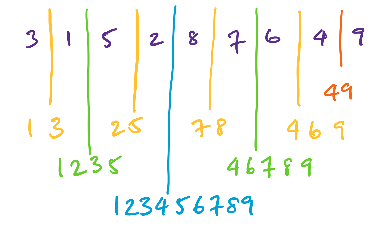
Here, we are given an array $[3,1,5,2,8,7,6,4,9]$ and we sort recursively, splitting the array in half each time. The results of each sort are then merged back together.
The algorithm in pseudocode is essentially the algorithm we described, with the addition of the base case of when your array is just a single element.
    \begin{algorithmic}
    \PROCEDURE{mergesort}{$A$}
        \STATE $n = $ size($A$)
        \IF{$n$ is 1}
            \RETURN{$A$}
        \ENDIF
        \STATE $m = \left\lfloor \frac n 2 \right\rfloor$
        \STATE $B = $ \CALL{mergesort}{$A[1,\dots,m]$}
        \STATE $C = $ \CALL{mergesort}{$A[m+1,\dots,n]$}
        \STATE $A' = $ \CALL{merge}{$B,C$}
    \RETURN{$A'$}
    \ENDPROCEDURE
    \end{algorithmic}
Let's consider the efficiency of the algorithm. This is the first algorithm we've seen in this class that's expressed recursively, and it's not necessarily immediately clear how to consider the running time. However, if we think about what the algorithm is really doing, the crucial operation we need to keep track of is comparisons. We'll use this as a proxy of the running time (technically, there are a few more constants floating about if we wanted to be more strict about counting operations).
Suppose $T(n)$ is the number of comparisons that Mergesort performs on an array of size $n$. Then, we have the following pieces of information:
- If $A$ only contains one element, then it doesn't perform any comparisons at all.
- Now, if $A$ is larger,
- Mergesort is run twice, on arrays of size about $\frac n 2$. This value is about $2 \cdot T(n/2)$.
- Merge is run once on two arrays of size about $\frac n 2$. This is up to $n$ comparisons.
What can we do with this? Let's run through a simplified case first. Suppose $n$ is a power of 2, so $n = 2^k$ for some $k \geq 0$. We can then express $T(n)$ as a recurrence,
\[T(n) = \begin{cases} 0 & \text{if $n = 1$,} \\
2 \cdot T\left(\frac n 2 \right) + n & \text{if $n \gt 1$.} \end{cases} \]
This is a nice recurrence. There's a problem, though: what is the asymptotic behaviour of this function?