Now, we can revise our pseudocode for Dijkstra's algorithm to make explicit some of the implementation choices we made.
    \begin{algorithmic}
    \PROCEDURE{Dijkstra}{$G,s$}
        \STATE $d[s] = 0, \pi[s] = \varnothing$
        \FORALL{$v \neq s$}
            \STATE $d[v] = \infty, \pi[v] = \varnothing$
        \ENDFOR
        \STATE Create empty priority queue $P$
        \FORALL{$v \in V$}
            \STATE \CALL{insert}{$P,(v,d[v])$}
        \ENDFOR
        \WHILE{$P$ is not empty}
            \STATE $u = $ \CALL{extract-min}{$P$}
            \FORALL{$(u,v) \in E$}
                \IF{$d[v] \gt d[u] + w((u,v))$}
                    \STATE \CALL{update}{$P,v,d[u] + w((u,v))$}
                    \STATE $d[v] = d[u] + w((u,v))$
                    \STATE $\pi[v] = u$
                \ENDIF
            \ENDFOR
        \ENDWHILE
    \ENDPROCEDURE
    \end{algorithmic}
Much of the additional logic is setting up all the data structures we need. The real question is what happens within the while loop.
Here, we use our priority queue $P$ to maintain the set of vertices that aren't explored yet. On each iteration, while there are still unexplored vertices, we take the vertex $v$ with minimal $d[v]$ out of the priority queue. We then update the keys (distances) for all the remaining unexplored vertices for the next iteration.
Dijsktra's algorithm when implemented with a binary heap priority queue has time complexity $O(m \log n)$, where $m = |E|$ and $n = |V|$.
Everything before the while loop is setting up the data structures we need for the algorithm. This takes $O(n)$ time, based on our discussions about arrays and priority queues.
Now, consider the while loop. We perform one iteration of the loop for each vertex $V$. In each iteration, we remove a vertex from the priority queue, which has cost $O(\log n)$. We also examine a number of edges. It is important to note that since we only examine outgoing edges of $u$, this means that across all iterations of the while loop, we only examine each edge once.
Putting that together, we have $n$ deletions from $P$ and at most $m$ updates to the priority queue. This gives us a total of $O(n) + O(n \log n) + O(m \log n)$ time. Therefore, Dijkstra's algorithm has time complexity $O(m \log n)$.
There is a caveat with this. One may wonder whether this is really better than using an array to hold the $r(v)$ values. Finding the minimum in this case requires $O(n)$ time to scan the array, which is clearly worse than $O(\log n)$. However, we can update the array in $O(1)$ time, which is better than $O(\log n)$. In this alternative implementation, we require $O(n^2)$ time for finding the minimum $r(v)$ and $O(m)$ time for updating the $r(v)$'s. Then we have $O(n^2) + O(m)$, which is still $O(n^2)$ and we're good, since $m \leq n^2$.
Hold on: if $m \leq n^2$, how does $O(n^2)$ compare with $O(m \log n)$? Wouldn't that mean that we really have $O(n^2 \log n)$ time for our priority queue implementation? And that is a very good question to ask, because it turns out that the complexity changes depending on how many edges you have. If you have few edges and $m$ is not close to $n^2$ (i.e. $G$ is a sparse graph), then the priority queue implementation wins out. But if your graph contains many edges and $m$ is closer to $n^2$ (i.e. $G$ is dense graph), the array implementation may be a better choice. Tricky!
However, it turns out we can do even better than this, by tinkering with the implementation of the priority queue itself. Recall that our implementation uses a binary heap to implement the priority queue, which has $O(\log n)$ time for all of its operations. One can squeeze out additional efficiency by using a Fibonacci heap, which were invented by Fredman and Tarjan in 1984. These heaps have an amortized running time of $O(1)$ for update(S,x,k), which means that our analysis of Dijkstra's algorithm improves to $O(m + n \log n)$. This implementation wins out no matter how many edges your graph has. You can read about Fibonacci heaps in CLRS Chapter 19.
This time, we'll be dealing with undirected graphs. Recall that a spanning tree is sort of a minimal connected subgraph for a connected graph.
Let $G = (V,E)$ be an undirected graph. Then a subgraph $H = (V',E')$ of $G$ is a spanning tree if $V' = V$ and $H$ is acyclic and connected (i.e. $H$ is a tree).
If we apply weights to the edges like we did with shortest paths, we get the following notion.
Given a connected undirected graph $G = (V,E)$ with a edge weight function $w:E \to \mathbb R^+$, a minimum spanning tree $T = (V,E')$ of $G$ is a spanning tree of $G$ such the sum of the edge weights is minimized.
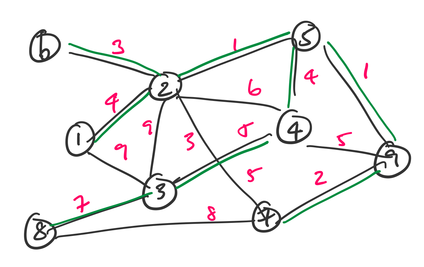
Consider the following graph.
A minimum spanning tree for this graph is given in green.
Just as the spanning tree represents a sort of minimal subgraph that remains connected, the minimum spanning tree is the least cost version of that. So imagine that we want to minimize the cost of travelling between all of these cities or rolling out connections.
The minimum spanning tree problem is: Given a graph $G = (V,E)$ with edge weight function $w : E \to \mathbb R^+$, find a minimum spanning tree $T$ for $G$.
One of the neat things about this problem is that we can actually remove the language about spanning trees and ask the simpler question of finding the least cost connected subgraph. The answer naturally leads to a minimum spanning tree (you can try to convince yourself of this fact).
We will look at two algorithms for the minimum spanning tree problem, both of which take a greedy approach. For simplicity, we will assume that no two edges have the same weight.
Prim's algorithm is named for Robert Prim, who proposed this algorithm in 1957 while he was at Bell Labs. However, the algorithm was previously published by Vojtěch Jarník in 1930 in Czech. I can relate, having unknowingly rediscovered a result that was previously published only in Hungarian.
Prim's algorithm is a natural starting point for us, because it turns out the idea behind it is very similar to Dijkstra's algorithm for finding shortest paths. We can roughly describe the algorithm as follows:
We'll leave the pseudocode to when we talk about implementation and running time. For now, let's convince ourselves that this strategy actually works. What isn't clear at this point is that doing this either gets us a minimum weight spanning tree or even a spanning tree at all. We'll need a few definitions to aid us here.
A cycle is a path with no repeated vertices or edges other than the start and end vertex.
A very important thing to remember about trees is that they are graphs that don't have any cycles. Recall the following useful properties of trees.
Let $T$ be a tree with $n$ vertices.
Consider the following tree.
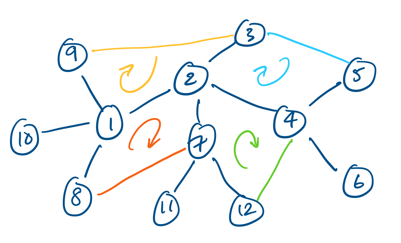
One can verify that it has exactly 11 edges and it is easy to see that removing any single edge will disconnect the graph. Some examples of possible edges that can be added between vertices are given in different colours and the cycles they create are highlighted.