To prove that a problem $A$ is $\mathbf{NP}$-complete,
- Show that $A \in \mathbf{NP}$. In other words, describe how to verify Yes instances of $A$ in polynomial time, by describing an appropriate certificate and how you would verify it.
- Choose a problem $B$ that you already know is $\mathbf{NP}$-complete.
- Describe how to map Yes instances of $B$ to Yes instances of $A$.
- Show that your mapping can be computed in polynomial time.
Let's try this out.
Satisfiability $\leq_P$ 3-SAT.
We need to transform an arbitrary boolean formula $\varphi$ into one that is in CNF and has at most three literals per clause. To do this, we will go through a series of transformations, each of which preserves the truth of the original formula.
First, we will parenthesize the formula into what is sometimes called a well-formed formula. Essentially, this means rewriting the formula so that the order of operations are explicitly defined by the parentheses. It is clear that this rewriting doesn't change the formula.
Once we have such a formula, we can very easily construct a parse tree for the formula. For example, for the formula $\varphi = (((x_1 \to x_2) \wedge (x_3 \wedge \neg x_1)) \vee (x_2 \to \neg x_4)) \vee x_3$, we have the following parse tree.
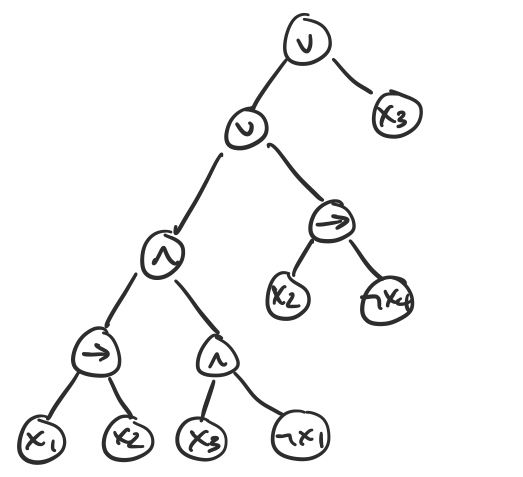
We observe that in such a tree, the leaves are all literals and the internal nodes of the tree are all connectives. We observe that every connective has exactly two children. What we will do is, for each connective $(x \circ y)$, construct a clause $(z \leftrightarrow x \circ y)$, where $z$ is a new variable and replace the subformula with $z$. Since all connectives are binary, we have a set of clauses with three literals of the form $(z \leftrightarrow x \circ y)$.
For each of these clauses, we can rewrite them using only $\vee$ and $\wedge$ by using a truth table and writing the result in disjunctive normal form (ors of ands). Since all of our clauses are of the form $C = (z \leftrightarrow (x \circ y))$, we have a truth table
| $x$ | $y$ | $z$ | $C$
|
|---|
| T | T | T | ?
|
| T | T | F | ?
|
| T | F | T | ?
|
| T | F | F | ?
|
| F | T | T | ?
|
| F | T | F | ?
|
| F | F | T | ?
|
| F | F | F | ?
|
Then we can construct a formula in disjunctive normal form for $\neg C$ by taking each row that evaluates to $F$, $\wedge$ing the variables together and $\vee$ing those clauses.
For example, suppose $C = (z \leftrightarrow (x \wedge \neg y))$. Then
| $x$ | $y$ | $z$ | $(z \leftrightarrow (x \wedge y))$
|
|---|
| T | T | T | T
|
| T | T | F | F
|
| T | F | T | F
|
| T | F | F | T
|
| F | T | T | F
|
| F | T | F | T
|
| F | F | T | F
|
| F | F | F | T
|
This gives us the formula
\[\neg C = (x \wedge y \wedge \neg z) \vee (x \wedge \neg y \wedge z) \vee (\neg x \wedge y \wedge z) \vee (\neg x \wedge \neg y \wedge z).\]
We then apply De Morgan's laws on our formula for $\neg C$ to turn the result into a formula for $C$ in conjunctive normal form. Again, this does not change the satisfiability of the formula.
This leaves us with clauses with three, two, or one literals. We can stuff the clauses with only one or two literals with dummy variables as follows:
- if we have a clause $(x_1 \vee x_2)$, replace it with $(x_1 \vee x_2 \vee p) \wedge (x_1 \vee x_2 \vee \neg p)$;
- if we have a clause $(x_1)$, replace it with $(x_1 \vee p \vee q) \wedge (x_1 \vee \neg p \vee q) \wedge (x_1 \vee p \vee \neg q) \wedge (x_1 \vee \neg p \vee \neg q)$;
where $p$ and $q$ are new variables. We use the same variables $p$ and $q$ for all clauses that need them. It is clear that adding these variables does not affect the satisfiability of the formula.
It remains to show that the construction can be done in polynomial time. It is clear that parenthesizing the formula can be done in one pass of the formula. Then what is the size of the parse tree? This looks like it could be exponential, but it's actually linear in the length of the formula: every node corresponds to either a literal or a connective in the formula. This is important, because we use the parse tree as the basis of our transformation.
Roughly speaking, we define a clause for each connective in our parse tree. This corresponds to one clause per internal node of the parse tree, which is linear in the length of the formula. Each clause increases the size of the instance by a constant amount. Then rewriting each clause also requires a constant amount of time and space: in the very worst case, we get a formula of eight clauses in DNF per clause we start out with.
In total, performing this transformation only increases the size of the formula linearly in the length of the original formula.
3-SAT is $\mathbf{NP}$-complete.
First, we need to show that 3-SAT is in $\mathbf{NP}$. An appropriate certificate for 3-SAT is an assignment of variables. This is a list $(x_1, x_2, \dots, x_n) = (T,F,T,\dots,F)$. We can then test each clause to see if it evaluates to $T$ or $F$. If all clauses evaluate to $T$, then our formula is satisfied by the given assignment. Otherwise, it isn't. The certificate is linear in the number of variables in the formula. This is clearly verifiable in polynomial time.
By Theorem 25.1, we have that Satisfiability $\leq_P$ 3-SAT. By Theorem 24.8, Satisfiability is $\mathbf{NP}$-complete. Therefore, 3-SAT is $\mathbf{NP}$-complete.
Then it is not too hard to see that by our previous reductions and a quick argument about how they can be efficiently verified, we also have that Independent Set, Vertex Cover, and Set Cover are all $\mathbf{NP}$-complete.
One question you might have is what about 4-SAT? That is probably not a question you have, but we can see that we can turn any 3-SAT formula into a 4-SAT formula by doing our dummy variable trick. The other question is what about 2-SAT?
It turns out 2-SAT is in $\mathbf P$! This was first shown by Krom in 1967. Intuitively, the reason for this is that since every clause is of the form $(x \vee y)$, what you can do is start setting variables and seeing what you get.
For example, if $x$ is set to True, then we're done, but if $x$ is False, in order for the clause to be True, $y$ must be True. Following this chain of implications is easy when you only have two literals per clause, since you have only one possibility and you can keep on going until you get a satisfying assignment or you get stuck. If you have three literals per clause, you get two possibilities and your choices start looking like a tree, leading to exponential blowup.
We immediately get the following.
The following problems are $\mathbf{NP}$-complete:
- Independent Set
- Vertex Cover
- Set Cover
By Proposition 17.12, if $A$ is $\mathbf{NP}$-complete, and $A \leq_P B$, and $B \in \mathbf{NP}$, then $B$ is $\mathbf{NP}$-complete. Therefore, it suffices to show that each of the problems is in $\mathbf{NP}$ and there exists a reduction from an $\mathbf{NP}$-complete problem. By Theorem 17.13, Satisfiability is $\mathbf{NP}$-complete.
- Independent Set is in $\mathbf{NP}$ by Proposition 17.9. We have 3-SAT $\leq_P$ Independent Set by Theorem 16.4 and 3-SAT is $\mathbf{NP}$-complete by Theorem 17.14(a). Therefore, Independent Set is $\mathbf{NP}$-complete.
- Vertex Cover is in $\mathbf{NP}$ by Proposition 17.9. We have Independent Set $\leq_P$ Vertex Cover by Proposition 15.10 and Independent Set is $\mathbf{NP}$-complete by Theorem 17.14(b). Therefore, Vertex Cover is $\mathbf{NP}$-complete.
- Set Cover is in $\mathbf{NP}$ by Proposition 17.9. We have Vertex Cover $\leq_P$ Set Cover by Proposition 15.13 and Vertex Cover is $\mathbf{NP}$-complete by Theorem 17.14(c). Therefore, Set Cover is $\mathbf{NP}$-complete.
Hamiltonian Cycle
Now, we'll prove something about a simple, but important graph problem. The following notion was due to the Irish mathematician William Rowan Hamilton in the early 1800s.
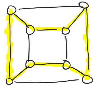
Let $G$ be a graph. A cycle is a Hamiltonian cycle if every vertex of $G$ is in the cycle. A path is a Hamiltonian path if every vertex of $G$ is in the path.
The following graph contains a Hamiltonian cycle that is highlighted.
Hamiltonian cycles and paths have some very interesting applications. One is a connection to Gray codes, which are a binary code on $n$ digits that are defined such that the successor of a number only has a one digit difference from the current number.
The obvious question that we can ask about Hamiltonian cycles is whether our graph contains one.
The Hamiltonian Cycle problem is: Given a graph $G$, does $G$ contain a Hamiltonian cycle?
There is are directed and undirected flavours of this problem. Let's start with a simple reduction.
Directed Hamiltonian Cycle $\leq_P$ Undirected Hamiltonian Cycle.
We'll describe the reduction informally. The big question is how to transform a directed graph into an undirected graph while maintaining the "directedness" of the edges. What we can do is split a vertex $v$ into three: $v_{in}, v, v_{out}$.
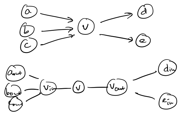
We join $v_{in}$ and $v$ by an edge and $v$ and $v_{out}$ by an edge. Then for all edges $(u,v)$, we join $u_{out}$ and $v_{in}$. It remains to show that there is a Hamiltonian cycle in one graph if and only if there is one in the other.
Here's another very interesting related problem.
The Traveling Salesman problem is: Given a list of $n$ cities, and costs $c(i,j) \geq 0$ for travelling from city $i$ to city $j$ and an integer $k \geq 0$, is there a sequence $i_1, i_2, \dots, i_n$ such that
\[\sum_{j=1}^n c(i_j, i_{j+1}) + c(i_n,i_1) \leq k?\]
Traveling Salesman is probably the most well-known example of an intractable problem: the idea is straightforward, it's easy to show that it's hard to solve, and it's easy to see why someone might possibly care about the problem.
The standard formulation of this problem doesn't involve graphs, but it's not hard to automatically interpret this as a problem on a complete graph of $n$ vertices. This view of the problem gives us an obvious reduction.
Hamiltonian Cycle $\leq_P$ Traveling Salesman.
We won't go through an entire formal proof, since the construction of the reduction is pretty simple. Let's describe how to take an instance of Hamiltonian Cycle, which is a directed graph $G$, and construct an instance of Traveling Salesman. An instance of Traveling Salesman is $(H,c,v)$, where $H$ is a complete graph with edge costs $c$, and $k \geq 0$.
If $G$ has $n$ vertices, we simply construct a complete graph on $n$ vertices and set $k = n$. Then we assign edge costs as follows: if $e$ is an edge of $G$, then $c(e) = 1$. Otherwise, $c(e) = 2$. Then all we need to do is show that the minimal cost Traveling Salesman tour with cost $n$ corresponds to the minimal cost Hamiltonian cycle if it exists, and there is no such tour if it doesn't, since to complete such a tour, we must include an edge with cost 2.
That was not so bad. Now, let's do something a bit more surprising: we'll show that 3-SAT reduces to Hamiltonian Cycle.