All that is left is to show that the path that we get from following successors from $s$ gets us the shortest $v,t$ path. Unlike with Dijkstra's algorithm, we haven't shown that it's not possible to create a cycle through our computation. This is something that we need to consider. First, let us consider the successor subgraph.
Let $G_s = (V,E_s)$ be the subgraph defined by \[E_s = \{(v,s[v]) \mid v \in V\}.\]
If the successor graph $G_s$ contains a cycle, it must be a negative cycle.
First, we observe that if $s[v] = x$, then we have that $d[v] \geq d[x] + w(v,x)$. Now, consider a cycle $C$ on $v_1, v_2, \dots, v_k, v_1$ in $G_s$ and assume that $(v_k,v_1)$ is the last edge that belongs to the cycle that is added to $G_s$.
At the point that $v_1$is assigned to $s[v_k]$ and added to $G_s$, we have the following inequalities: \begin{align*} d[v_1] & \geq d[v_2] + w(v_1,v_2) \\ d[v_2] & \geq d[v_3] + w(v_2,v_3) \\ & \vdots \\ d[v_{k-1}] & \geq d[v_k] + w(v_{k-1},v_k) \\ d[v_k] & \gt d[v_1] + w(v_k,v_1) \\ \end{align*} Adding these inequalities together and grouping the $d[i]$'s on one side and edge weights on the other gives us \begin{align*} d[v_1] + \cdots + d[v_k] - d[v_1] - \cdots d[v_k] &\gt w(v_1,v_2) + \cdots + w(v_k,v_1) \\ 0 &\gt w(v_1,v_2) + \cdots + w(v_k,v_1) \\ 0 &\gt w(C) \\ \end{align*}
So if our graph does not have any negative cycles, then we will not end up with a cycle in our successor graph. It remains to show that the paths that are obtained via the successor graph are actually the shortest paths from $v$ to $t$.
Assuming no negative cycles, Bellman-Ford finds shortest $v,t$ paths for every vertex $v$ in $O(mn)$ time and $O(n)$ space.
Since there are no negative cycles, the successor graph $G_s$ cannot contain any cycles. Therefore, the successor graph must consist of paths to $t$. Consider a path $P$ on vertices $v = v_1, v_2, \dots, v_k = t$.
Once the algorithm terminates, if $s[v] = x$, we must have $d[v] = d[x] + w(v,x)$ for all vertices $v \in V$. This gives us the equations \begin{align*} d[v_1] & = d[v_2] + w(v_1,v_2) \\ d[v_2] & = d[v_3] + w(v_2,v_3) \\ & \vdots \\ d[v_{k-1}] & = d[v_k] + w(v_{k-1},v_k) \\ \end{align*} Since $v_1 = v$ and $d_k = t$, adding these equations together gives us \begin{align*} d[v] &= d[t] + w(v_1,v_2) + \cdots + w(v_{k-1},v_k) \\ &= 0 + w(v_1,v_2) + \cdots + w(v_{k-1},v_k) \\ &= w(P) \\ \end{align*} By Proposition 16.6, $d[v]$ is the weight of the shortest path from $v$ to $t$, so $P$ is the shortest path from $v$ to $t$.
So Bellman-Ford is able to compute the shortest path, assuming there are no negative cycles. And that's fine, because we know that if a graph has a negative cycle, then it doesn't have a shortest path.
In the following, $\Sigma$ will denote a finite alphabet of symbols. For example, $\{0,1\}$ is the binary alphabet and $\{A,C,G,T\}$ is the DNA alphabet. We denote the set of strings over a particular alphabet $\Sigma$ by $\Sigma^*$. So $\{0,1\}^*$ denotes the set of all binary strings.
One of the key insights that led to the development of bioinformatics was the observation that we could view sequences of DNA and RNA as strings. If we take a formal language-theoretic view of this, we can treat DNA and RNA as strings over a four-letter alphabet: $\{A,C,G,T\}$ for DNA and $\{A,C,G,U\}$ for RNA.
This simplifies the behaviour of DNA and RNA a bit. After all, they aren't just sequences, they have various biochemical properties as well. For instance, DNA is double-stranded and any sequence we read is really just one side of a double-stranded sequence. If we consider a DNA sequence $s \in \{A,C,G,T\}^*$, we can define its Watson-Crick complement mathematically.
We say that a function $h : \Sigma^* \to \Sigma^*$ is a homomorphism if $h(w)$, with $w \in \Sigma^*$ satisfies the following:
Informally, homomorphisms are string functions that map each letter to a string while preserving the order of the string. Homomorphisms are a definition derived from algebraic structures (that is, there are ring homomorphisms, group homomorphisms, etc., and this is because strings themselves form an algebraic structure called a monoid). This definition leads us to the actual notion we care about: antimorphisms.
We say that a function $\psi : \Sigma^* \to \Sigma^*$ is an antimorphism if $\psi(w)$, with $w \in \Sigma^*$ satisfies the following:
In other words, an antimorphism is like a homomorphism in that it maps each letter of a string to another string, but it preserves the order in reverse. This is exactly what for a definition of the complement of a DNA sequence.
The Watson-Crick antimorphism is the involutive antimorphism $\theta: \{A,C,G,T\}^* \to \{A,C,G,T\}^*$ defined by $\theta(A) = T$, $\theta(C) = G$, $\theta(G) = C$, $\theta(T) = A$.
So for any string $s \in \{A,C,G,T\}^*$, $\theta(s)$ is the Watson-Crick complement of $s$. This has the additional nice property of being an involution: $\theta(\theta(s)) = s$, or the fact that applying the function twice gets us the identity.
We can get a similar definition for the RNA alphabet $\{A,C,G,U\}$, where $U$ takes the same role as $T$ in our theoretical model. Unlike DNA, RNA is not double-stranded, but it can still bind to itself, which creates what are called secondary structures.
Obviously, strings are one-dimensional objects, but it is possible to predict the formation of secondary structures using sequences of RNA. There are some very nice combinatorial definitions for what this looks like.
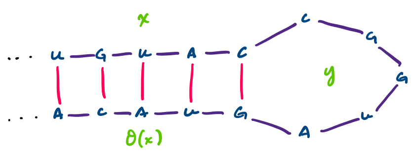
Consider the RNA sequence $UGUACCGGUAGUACA$. This sequence can have the following secondary structure.
This particular structure is called a hairpin. Notice that we can write it as a string $xy\theta(x)$, where $x = UGUAC$ and $y = CGGUA$. Generally, hairpins can be said to have this sequence structure $uv\theta(u)$, where $u,v \in \Sigma^*$. In this way, we can identify secondary structures combinatorially on one-dimensional sequences.
The specific problem we would like to work on is prediction: which secondary structures are most likely to form given an RNA sequence. We will use the following definition/restrictions.
A secondary structure on a string $w = b_1 \cdots b_n$ of length $n$ over the alphabet $\{A,C,G,U\}$ is a set of pairs $S = \{(i,j)\}$, where $i,j \in \{1,\dots,n\}$ such that
Our algorithm, due to Ruth Nussinov in her PhD thesis in 1977 and published later with Jacobson in 1980, is based on the idea that the secondary structure most likely to occur is the one with the most base pairs. This means that our problem is a maximization problem.
The RNA secondary structure prediction problem is: given an RNA sequence $w = b_1 b_2 \cdots b_n$, determine a secondary structure $S$ with the maximum number of base pairs.