CMSC 27200 — Lecture 16

Recall from Lecture 6 that we were interested in solving the shortest path problem, where we are given a digraph $G$ with edge weights, a source vertex $s$ and a destination vertex $t$. We saw how to solve this using a greedy approach. Now, we are ready to revisit a problem that we were introduced to earlier that we couldn't solve: how to find the shortest path in a graph that contains negative edge weights.

One of the things some of you observed was that if there's a negative cycle (i.e. a cycle for which the sum of its edge weights is negative) on a path from $s$ to $t$, then there's no shortest path from $s$ to $t$. The proof is not complicated: if there's a negative cycle, then we can take the negative cycle as much as we like to decrease the cost of the path by an arbitrary amount.

Now, we will consider a non-greedy approach (read: dynamic programming) to solving the problem that will allow us to use negative edge weighs. Our algorithm will even be able to determine whether any of our paths contain a negative cycle, so we can figure out whether there a shortest path exists.

Rather than computing the shortest path from a source $s$ to every other node, we consider sort of the backwards version of the problem, where we compute the shortest path from every vertex to our destination $t$.

The single-destination shortest-paths problem is: Given a directed graph $G = (V,E)$ with an edge weight function $e: E \to \mathbb R$ and a destination vertex $t$, find a shortest path from $v$ to $t$ for every $v \in V$.

Because we plan to use dynamic programming, we need to determine what subproblem is appropriate to compute in the service of finding a shortest path. Here, we can take some inspiration from our greedy approach: recall that Dijkstra's algorithm kept an estimated weight of the path from the source $s$ to each vertex $v$.

To help clarify this decision, here is a useful result that we won't prove but is similar to something you may have seen in discrete math.

Suppose $G$ has no negative cycles. Then there is a shortest path from $u$ to $v$ that does not repeat any vertices.

One consequence of this result is that any shortest path will have at most $n-1$ edges in it, since any path that has more edges will revisit some vertex.

We will define $OPT(i,v)$ to be the weight of a shortest path from $v$ to $t$ that uses at most $i$ edges. So if we want to compute the shortest path from $s$ to $t$, we would want to compute $OPT(n-1,s)$.

Let us consider a shortest path from a vertex $v$ to our destination $t$, which would have weight $OPT(i,v)$. How can we decompose this path? Since we want to express this in terms of some shorter path, it makes sense to consider the first edge in our path, say $(v,x)$, followed by the shortest path from that vertex $x$ to $t$. So we have the following possibilities.

As usual, the recurrence leads us to a straightforward algorithm that fills out a table.

    \begin{algorithmic}
    \PROCEDURE{shortest-paths}{$G,t$}
        \FORALL{$v \in V$}
            \STATE $P[0,v] \gets \infty$
        \ENDFOR
        \STATE $P[0,t] \gets 0$
        \FOR{$i$ from $1$ to $n-1$}
            \FORALL{$v \in V$}
                \STATE $P[i,v] \gets P[i-1,v]$
                \FORALL{$(v,x) \in E$}
                    \STATE $P[i,v] \gets \min\{P[i,v], P[i-1,x]+w(v,x)\}$
                \ENDFOR
            \ENDFOR
        \ENDFOR
    \ENDPROCEDURE
    \end{algorithmic}

This algorithm is pretty straightforward. The tricky part is counting the number of iterations this algorithm makes. Just like with Dijkstra's algorithm, it's easy to conclude that there must be something like $O(mn^2)$ just by looking at the definition of the loops, but if we observe how the edges are chosen, we see that only edges the leave a particular vertex are examined at each iteration, so every edge is examined at most once. So the inner two loops together comprise a total of $O(m)$ iterations. In total, this gives us $O(mn)$ time.

On the other hand, the algorithm clearly requires $O(n^2)$ space. This seems like a lot, especially compared to Dikjstra's algorithm. It turns out that we can do better by applying some of the same ideas.

Bellman-Ford

One observation we can make is that in the end, we really don't care how many edges a shortest path actually uses. In that sense, all we really need to do is keep track of the minimum weight of the path from each vertex. So instead of keeping track of a table of size $O(n^2)$, we can keep track of an array $d$ of estimated weights of shortest paths.

The problem with this is that this may not be enough information to reconstruct the actual path itself. We take a similar approach to Dijkstra's algorithm and keep track of the successors for each vertex as we update the estimated weights $d$. In doing so, we reduce our space requirements from a table of size $O(n^2)$ to two arrays of size $n$, which is $O(n)$.

This leads to the following algorithm attributed to Bellman, who we saw earlier as the inventor of dynamic programming, and Ford, who we will see again very shortly when we get into network flows. But even though the algorithm is called Bellman-Ford, they didn't publish together: Ford published the algorithm in 1956, while Bellman published it in 1958. Even this isn't the only instance: Moore also published the algorithm in 1957 and sometimes also gets attribution, while Shimbel published it in 1955 and does not.

    \begin{algorithmic}
    \PROCEDURE{bellman-ford}{$G,t$}
        \FORALL{$v \in V$}
            \STATE $d[v] \gets \infty$
            \STATE $s[v] \gets \varnothing$
        \ENDFOR
        \STATE $d[t] \gets 0$
        \FOR{$i$ from $1$ to $n-1$}
            \FORALL{$x \in V$}
                \IF{$d[x]$ was updated in the previous iteration}
                    \FORALL{$(v,x) \in E$}
                        \IF{$d[v] \gt d[x] + w((v,x))$}
                            \STATE $d[v] \gets d[x] + w(v,x)$
                            \STATE $s[v] \gets x$
                        \ENDIF
                    \ENDFOR
                \ENDIF
            \ENDFOR
        \ENDFOR
    \ENDPROCEDURE
    \end{algorithmic}

The running time of this algorithm is still $O(mn)$ by the same argument as before and the space requirements have clearly changed to $O(n)$. What is not as obvious is that $d$ ends up holding the weights of the shortest paths for each vertex and that $s$ correctly holds the successor for each vertex. First, we will show that Bellman-Ford correctly computes the weight of the shortest path.

After the $i$th iteration of the outer loop of Bellman-Ford, the following properties hold for every vertex $v \in V$:

We will prove this by induction on $i$. First, we consider $i = 0$. We have $d[t] = 0$ and $d[v] = \infty$ for all $v \neq t$, since there are no paths from $v$ to $t$ with 0 edges.

Now consider $i \gt 0$ and consider an update to $d[v] = d[x] + w(v,x)$. By our inductive hypothesis, $d[x]$ is the weight of a path from $x$ to $t$, so $d[x] + w(v,x)$ is the weight of a path from $v$ to $t$. So (1) holds.

Now, consider a shortest path $P$ from $v$ to $t$ with at most $i$ edges. Let $x$ be the first vertex after $v$ in $P$. Then the subpath $P'$ from $x$ to $t$ is a path from $x$ to $t$ with at most $i-1$ edges.

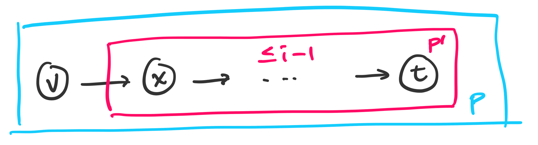
By our inductive hypothesis, $d[x]$ is the weight of a shortest path from $x$ to $t$ with at most $i-1$ edges after $i-1$ iterations of the outer loop of Bellman-Ford. So $d[x] \leq w(P')$.

Then on the next iteration, we consider the edge $(v,x)$. We have \[d[v] \leq d[x] + w(v,x) \leq w(P') + w(v,x) = w(P).\] So after $i$ iterations, $d[v]$ is at most the weight of the shortest path from $v$ to $t$ with at most $i$ edges. So (2) holds.

CMSC 27200 — Lecture 16

Shortest paths, revisited

Bellman-Ford