Let's consider the efficiency of mergesort. This is our first recursive algorithm, and it's not necessarily immediately clear how to consider the running time. However, if we think about what the algorithm is really doing, the crucial operation we need to keep track of is comparisons. We'll use this as a proxy of the running time (technically, there are a few more constants floating about if we wanted to be more strict about counting operations).
Suppose $T(n)$ is the number of comparisons that Mergesort performs on an array of size $n$. Then, we have the following pieces of information:
What can we do with this? Let's run through a simplified case first.
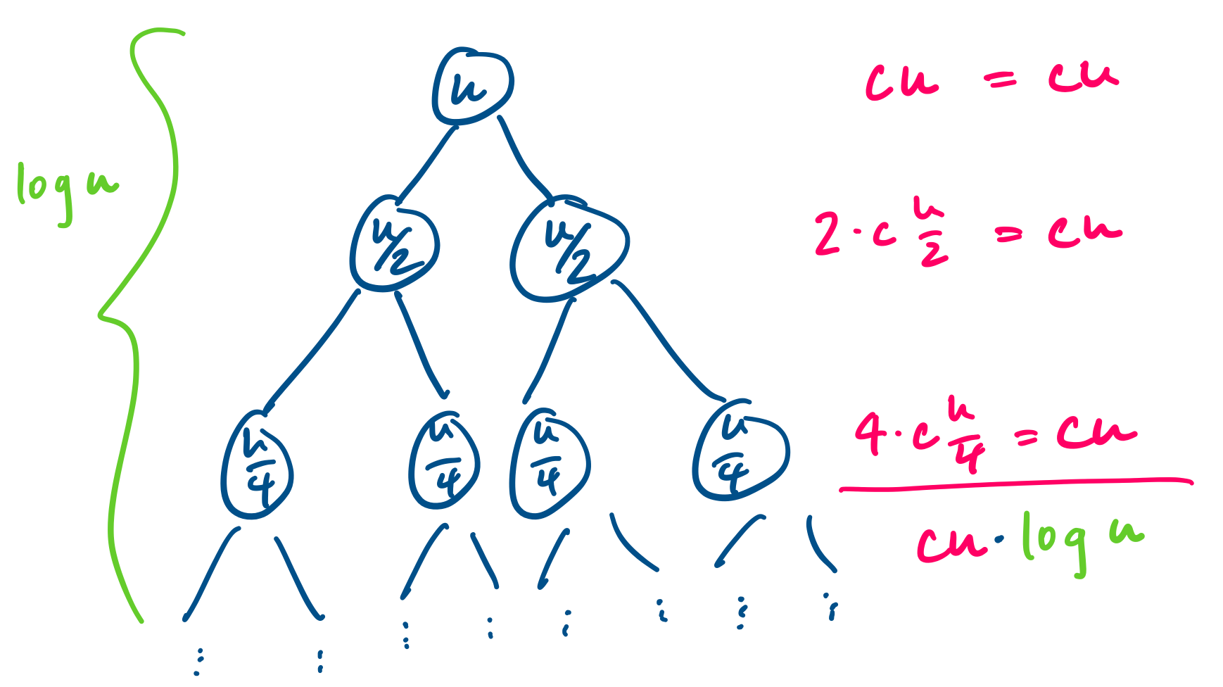
Suppose $n$ is a power of 2, so $n = 2^k$ for some $k \geq 0$. We can then express $T(n)$ as a recurrence, \[T(n) = \begin{cases} 0 & \text{if $n = 1$,} \\ 2 \cdot T\left(\frac n 2 \right) + n & \text{if $n \gt 1$.} \end{cases} \]
This is a relatively simple recurrence to solve and we have a few ways of looking at it. We can try to gain some insight by expanding our tree of subproblems.
We can then use this to come up with a guess for our recurrence, or if we prefer, we can try iterating the recurrence or guessing the first few values. Here's what we get from iterating: \begin{align*} T(2^k) &= 2 \cdot T(2^{k-1}) + 2^k \\ &= 2 \cdot (2 \cdot T(2^{k-2}) + 2^{k-1}) + 2^k \\ &= 2^2 \cdot T(2^{k-2}) + 2^k + 2^k \\ &= 2^2 \cdot (2 \cdot T(2^{k-3}) + 2^{k-2}) + 2^k + 2^k \\ &= 2^3 \cdot T(2^{k-3}) + 2^k + 2^k + 2^k \\ & \vdots \\ &= 2^j \cdot T(2^{k-j}) + j 2^k \\ & \vdots \\ &= 2^k \cdot T(1) + k 2^k \\ &= k 2^k \end{align*} We can then take our hypothesis and prove the recurrence formally using induction. Once we've proved it, we notice that this works out very nicely, because notice that $k = \log_2 2^k$ and since $n = 2^k$, we get $T(n) = O(n \log n)$.
Of course, this recurrence works for $n$ which are exact powers of 2. What about all of those numbers that aren't so lucky? If we re-examine our algorithm for Mergesort, we notice that it's possible that we might not get to break our array clean in half, in which case one subarray has size $\lfloor n/2 \rfloor$ and the other has size $\lceil n/2 \rceil$. We would need to rewrite our recurrence as follows \[T(n) \leq \begin{cases} 0 & \text{if $n = 1$,} \\ T\left(\left\lfloor \frac n 2 \right\rfloor\right) + T\left(\left\lceil \frac n 2 \right\rceil \right) + n & \text{if $n \gt 1$.} \end{cases} \]
Of course, since we care about upper bounds, this doesn't really matter and we can make things more convenient by smoothing out those annoying details. This recurrence is still sufficient to give us the following result.
$T(n)$ is $O(n \log n)$.
If you are really motivated to prove this with floors and ceilings, it is certainly possible. You would need to play around with the recurrence and somehow guess your way into finding $T(n) \leq n \lceil \log n \rceil$ and then proving that this holds by induction on $n$.
This was a bit of an ad-hoc refresher of how to deal with recurrences. However, if guessing and checking makes you uneasy, we will take a look at a more powerful result that lets us avoid this.
So far, the recurrences we've run into are not terribly complicated and so could afford to be pretty ad-hoc with how we've dealt with them. Eventually, we will be running into situations where we need to divide our problem into more than two subproblems, which will result in more complicated recurrences. Fortunately, there is a bit of a reliable result that covers most of the types of recurrences we're likely to see.
In algorithms analysis, the form of recurrence we tend to see is the following.
A divide-and-conquer recurrence is a recurrence of the form \[T(n) = a T\left(\frac n b\right) + f(n)\] where $a$ is the number of subproblems, $b$ is the factor by which we decrease the size of the subproblem, and $f(n)$ is the cost of combining solutions to subproblems.
We can gain some intuition about how to work with this by looking at its associated recursion tree. For convenience, we assume that $n$ is a power of $b$. Then at each level, each problem breaks into $a$ subproblems. What this means is that on the $i$th level of the tree, we have a total of $a^i$ subproblems, each of size $\frac{n}{b^i}$. In total, we will have $1 + \log_b n$ levels. Now, suppose also that we have $f(n) = n^c$ for some fixed constant $c$ (please ignore the fact that the illustration says $k$). We have the following.
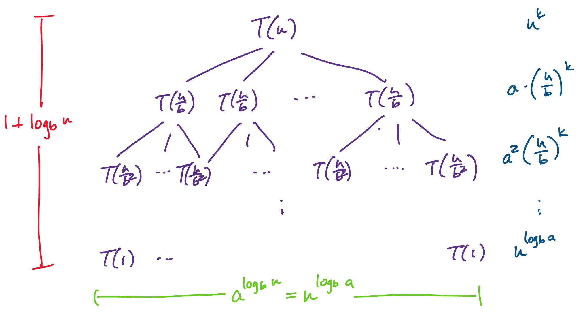
Adding all of these up, we have \[T(n) = \sum_{i=0}^{\log_b n} a^i \left( \frac{n}{b^i} \right)^c = n^c \sum_{i=0}^{\log_b n} \left(\frac{a}{b^c}\right)^i.\]
We would like to know what the asymptotic behaviour of this recurrence is. This will depend on what $a,b,c$ are, which will determine which term of $T(n)$ dominates.
Taking $r = \frac{a}{b^c}$ and $k = \log_b n$ together with the fact that $\frac{a}{b^c} \lt 1$ if and only if $c \gt \log_b a$, we arrive at the following.
Let $a \geq 1, b \geq 2, c \geq 0$ and let $T:\mathbb N \to \mathbb R^+$ be defined by \[T(n) = aT\left(\frac n b\right) + \Theta(n^c), \] with $T(0) = 0$ and $T(1) = \Theta(1)$. Then, \[ T(n) = \begin{cases} \Theta(n^{\log_b a}) & \text{if $c \lt \log_b a$}, \\ \Theta(n^c \log n) & \text{if $c = \log_b a$}, \\ \Theta(n^c) & \text{if $c \gt \log_b a$}. \\ \end{cases} \]
This is called the Master Theorem in CLRS because it magically solves many of the divide and conquer recurrences we see and because most instructors don't really get into the proof. Observe that I skillfully avoided many details. But the origins of this particular recurrence and its solutions is due to Bentley, Haken, and Saxe in 1980, partly intended for use in algorithms classes. If you are really interested in the entirety of the proof, then you should take a look at CLRS 4.6.
Recall our recurrence from Mergesort. Let $T(n) = 2T\left(\frac n 2\right) + kn$, for some constant $k$. Here, we have $a = 2$, $b = 2$, and $c = 1$. Since $\log_2 2 = 1$, we have that $T(n)$ is $O(n \log n)$.
Now consider something like $T(n) = 3T\left(\frac n 2\right) + kn$. Here, we have $1 \lt \log_2 3 \lt 1.58$, so this gives us $T(n) = O(n^{\log_2 3}) = O(n^{1.58})$, a noticeable difference just by increasing the number of subproblems by 1.