 We claim that the probability of each outcome is simply the product of the edge weights on the path corresponding to the outcome. We will justify this shortly.
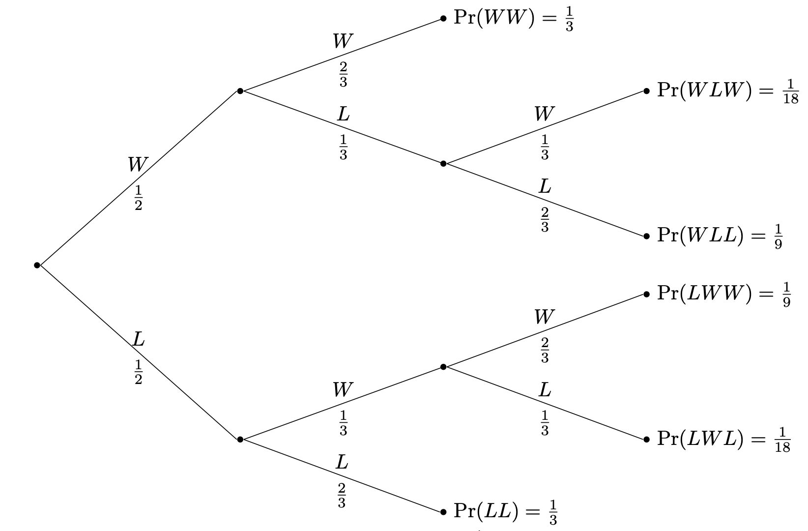
One helpful way of managing the information for a conditional probability problem is to use a tree diagram. We'll demonstrate via an example.
Volleyball matches can be played as a best-of-3 sets. Consider Team 🐦⬛, which when playing a match against their good friends, Team 🐈, has equal odds at winning the first set—that is, probability $\frac 1 2$. However, the probability that they win the following sets are determined by how well they did in the set prior. If 🐦⬛ wins a set, then they ride the momentum and go into the next set with probability $\frac 2 3$ of winning. However, if 🐦⬛ loses a set, then they are demoralized and go into the following set with probability $\frac 1 3$ of winning. What is the probability that 🐦⬛ wins the match against 🐈, given that 🐦⬛ loses the first set?
Let's apply the usual method.
We claim that the probability of each outcome is simply the product of the edge weights on the path corresponding to the outcome. We will justify this shortly.
Why does drawing a tree and multiplying the edge weights work to compute the outcome probabilities? Recall that by definition, we have that $\Pr(A \mid B) = \frac{\Pr(A \cap B)}{\Pr(B)}$. Rearranging this gives us $\Pr(A \cap B) = \Pr(A \mid B) \cdot \Pr(B)$. When viewed as a tree, the probability that a child event occurs is conditioned on the parent (and ancestors) event occurring.
For example, the probability that 🐦⬛ wins the first set is $\Pr(W_1) = \frac 1 2$ and the probability that they win the second set given that they win the first set is $\Pr(W_2 \mid W_1) = \frac 2 3$. So the probability that they do win both the first and second sets is $\Pr(W_1 \cap W_2) = \Pr(W_1) \cdot \Pr(W_2 \mid W_1)$.
So we simply multiply the probabilities along the path. But obviously, for this to work, this needs to be generalized. For instance, if we want to compute the probability along a path of length 3, then we have the following.
If $A,B,C$ are events, then \[\Pr(A \cap B \cap C) = \Pr(A) \cdot \Pr(B \mid A) \cdot \Pr(C \mid A \cap B).\]
The interpretation of this is that the probability that $A$ and $B$ and $C$ occurs is the probability that $C$ occurs given that both $A$ and $B$ occur together with the probability that they do, i.e. \[\Pr(C \mid A \cap B) \cdot \Pr(A \cap B).\] But the probability that $A$ and $B$ occur is just $\Pr(A) \cdot \Pr(B \mid A)$. One can formally extend this further to $n$ events to get our trick.
This highlights a trickiness when it comes to thinking about probability. We often think of events and conditioning as things that happen in sequence or over time. This is reflected in the way that we set up our problems. So it's important to remember that probability does not involve time at all. Mathematically speaking, all we have are sets of outcomes. This means that we can ask questions like the following.
Suppose our volleyball team 🐦⬛ won their match against 🐈. What is the probability that they lost the first set? This is the reverse of the problem we just solved. At first, it seems like a weird question to ask, because if we know they won, then we can probably just see whether they took the first set or not. But again, time is not something that we can express via probability theory. One way to think about this is that if the only information that we knew was that 🐦⬛ won the match, we can consider how likely it is that they won the first set.
Again, since we're just dealing with sets of outcomes, this question does have an answer. Recall that our events are winning the match: $W_{\mathrm{all}} = \{WW, WLW, LWW\}$, and losing the first set $L_1 = \{LL, LWL, LWW\}$. So we want $\Pr(L_1 \mid W_{\mathrm{all}})$, which is \[\Pr(L_1 \mid W_{\mathrm{all}}) = \frac{\Pr(L_1 \cap W_{\mathrm{all}})}{\Pr(W_{\mathrm{all}})} = \frac{\frac{1}{9}}{\frac 1 3 + \frac 1 {18} + \frac{1}{9}} = \frac 2 9.\]
An interesting observation one can make is that the two probabilities $\Pr(A \mid B)$ and $\Pr(B \mid A)$ are related, via $\Pr(A \cap B)$. Another way of thinking about this that if you know that both $A$ and $B$ occurred, it makes sense to consider the probability of either event relativeto the other. This observation was made by Bayes in the 1700s.
Let $A$ and $B$ be events. Then \[\Pr(A \mid B) = \frac{\Pr(B \mid A) \cdot \Pr(A)} {\Pr(B)}.\] This follows from the observation that $\Pr(A \cap B) = \Pr(B \mid A) \cdot \Pr(A)$. Since intersection is symmetric, $A \cap B$ we can use it to interpret conditioning on $A$ or $B$ and relate the two pairs of conditional probabilities.
Bayes' Theorem is often used in conjunction with the following result.
Let $A$ and $B$ be events. Then \[\Pr(A) = \Pr(A \mid B) \cdot \Pr(B) + \Pr(A \mid \overline B) \cdot \Pr(\overline B).\]
The Law of Total Probability is actually fairly straightforward: the probability of an event $A$ is the probability that it occurs given that some event $B$ occurs together with the probability that it occurs given that $B$ didn't occur. In other words, if you're in a situation where you may have "pieces" of information about the probability of $A$, it's possible to stitch them together to get a complete picture for $\Pr(A)$. And while this theorem is stated in terms of a single event $B$, it is possible to generalize this to a collection of events $B_1, \dots, B_k$ that partition the sample space.
Given a partition $B_1, \dots, B_k$ of $\Omega$ and an event $A$, \[\Pr(A) = \sum_{i=1}^k \Pr(A \mid B_i) \cdot \Pr(B_i).\]
Suppose it is board game night and we need to pick up some dice for our game. Unfortunately, whoever procured the dice did not do a very good job and about 5% of the dice are biased in the following way: $\Pr(1) = \frac 3 4$ and $\Pr(\omega) = \frac1{20}$ for $\omega = 2,3,4,5,6$. The other 95% of dice are plain old regular fair dice, but you have no way of figuring out whether you have a biased or fair die just on inspection. So, let's test them. If you pick up a die at random and roll two 1s, what is the probability that the die you picked up is biased?
What we essentially want to do is compute the probability that, given that we rolled two 1s, we picked up a biased die. If we let $B$ denote the event that we picked up a biased die and we denote by $R_{1,1}$ the event that we rolled two 1s, then we want to compute $\Pr(B \mid R_{1,1})$. Bayes' Theorem tells us that $$\Pr(B \mid R_{1,1}) = \frac{\Pr(R_{1,1} \mid B) \cdot \Pr(B)}{\Pr(R_{1,1})}.$$ We know $\Pr(B) = 5\% = \frac 1 {20}$ and we know that $\Pr(R_{1,1} \mid B) = \left( \frac 3 4 \right)^2 = \frac{9}{16}$. All we need to do is to calculate $\Pr(R_{1,1})$.
Recall that the Law of Total Probability tells us that $$\Pr(R_{1,1}) = \Pr(R_{1,1} \mid B) \cdot \Pr(B) + \Pr(R_{1,1} \mid \overline B) \cdot \Pr(\overline B)$$ where $\overline B$ is the non-biased die event, or in other words, the fair dice. This gives us \begin{align*} \Pr(R_{1,1}) &= \Pr(R_{1,1} \mid B) \cdot \Pr(B) + \Pr(R_{1,1} \mid \overline B) \cdot \Pr(\overline B) \\ &= \frac{9}{16} \cdot \frac 1{20} + \frac 1{36} \cdot \frac{19}{20} \\ &= \frac{157}{2880} \end{align*} Then going back to the formula from Bayes' Theorem, we have $$\Pr(B \mid R_{1,1}) = \frac{\frac{9}{320}}{\frac{157}{2880}} = \frac{81}{157} \approx 0.516.$$ So there's a pretty good chance that the die you got was biased. One or two more rolls will make it even more clear whether or not this is the case.
This looks fairly complicated, but we can still organize our problem as a tree diagram and get the same information.
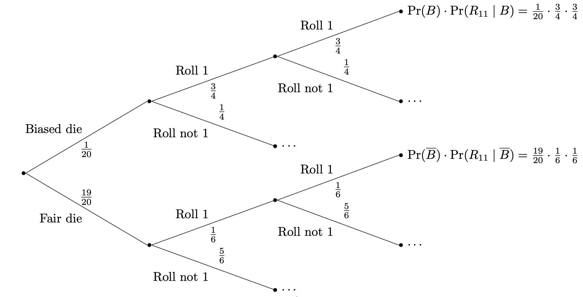
What's interesting about this is how the tree diagram naturally captures the ideas behind definitions like conditional probability and results like the law of total probability. For instance, it's clear from this diagram that we can just get the probability of rolling two 1's by looking at the resulting branches.