The Binomial Theorem
Let's think about binomials. This will seem like out of left field, but there is a connection, I promise. Recall that a binomial is an expression of two terms.
Hopefully, we are all familiar with how to expand a binomial. For instance, we have
$$(x+y)^2 = x^2 + xy + xy + y^2 = x^2 + 2xy + y^2.$$
Of course, we can do the same thing with higher degrees, like
\begin{align*}
(x+y)^3 &= (x+y)^2 (x+y) \\
&= (x^2 + 2xy + y^2)(x+y) \\
&= x^3 + 2x^2y + xy^2 + x^2y + 2xy^2 + y^3 \\
&= x^3 + 3x^2y + 3xy^2 + y^3
\end{align*}
Now, this process is straightforward but a bit tedious. Perhaps there is an alternative way to think about the resulting coefficients. This becomes a bit more clear if we step away from our algebraic impulses a bit. We can write
\begin{align*}
(x+y)^4 &= (x+y)(x+y)(x+y)(x+y) \\
&= xxxx + xxxy + xxyx + xxyy + xyxx + xyxy + xyyx + xyyy + \\
&\quad\: yxxx + yxxy + yxyx + yxyy + yyxx + yyxy + yyyx + yyyy
\end{align*}
When written in this way, each term looks much more like the kinds of objects that we've been working with over the past week. That is, we can think of each term as a combination of the terms from each binomial. In other words, how many terms of the form $x^3y$ are there? Exactly as there are many ways to choose three $x$'s and one $y$ from each binomial. This leads us to the following result.
For all $n \in \mathbb N$,
$$(x+y)^n = \sum^n_{j=0} \binom n j x^{n-j} y^j.$$
One can prove this via induction and it makes a nice exercise. We will prove this via a combinatorial argument similar to the above. Each term of our polynomial is of the form $x^{n-j}y^j$. Then the coefficients are exactly the number of ways to choose $n-j$ $x$'s from each binomial. There are $\binom n {n-j}$ ways to do this and $\binom n {n-j} = \binom n j$.
An interesting consequence of this theorem is how it gives us a connection between combinatorics and algebra. Being able to shift problems from one area of math to another is a powerful move because it allows us to use tools in different area of mathematics. In a class with more time to spend on combinatorics, we would have seen that this idea leads to generating functions, which are encodings of sequences as power series.
Suppose you have to prove the inductive case in some proof and you're faced with expanding $(k+1)^5$. Luckily, you don't need to futz around with expanding this polynomial and can directly apply the binomial theorem:
\begin{align*}
(k+1)^5 &= \binom 5 0 k^5 1^0 + \binom 5 1 k^4 1^1 + \binom 5 2 k^3 1^2 + \binom 5 3 k^2 1^3 + \binom 5 4 k 1^4 + \binom 5 5 k^0 1^5 \\
&= k^5 + 5k^4 + 10k^3 + 10k^2 + 5^k + 1
\end{align*}
This example suggests the following result, which follows from the Binomial Theorem by setting $y = 1$.
For all $n \in \mathbb N$,
$$(x+1)^n = \sum_{i=0}^n \binom n i x^i.$$
The following is a neat consequence of the binomial theorem that should match with our intution about what the binomial coefficients mean.
For all $n \in \mathbb N$,
$$\sum_{i=0}^n \binom n i = 2^n.$$
We have
$$2^n = (1+1)^n = \sum_{i=0}^n \binom n i 1^{n-i} 1^i = \sum_{i=0} \binom n i.$$
Of course, this makes total sense: if $\binom n i$ is the number of subsets of $n$ elements of size $i$, then adding the number of these subsets together is the total number of subsets of a set of size $n$, which is $2^n$.
There are a lot of other neat results that fall out of the Binomial Theorem. Perhaps the most famous one is due to Blaise Pascal in the 1600s.
For all natural numbers $n \geq k \gt 0$,
$$\binom{n+1}{k} = \binom{n}{k-1} + \binom n k.$$
As has been the case throughout this part of the course, there is a straightforward algebraic proof of this fact as well as a combinatorial proof. We will go through the combinatorial argument.
Let $A$ be a set of $n+1$ elements. We want to count the number of subsets of $A$ of size $k$, which is $\binom{n+1}{k}$.
Choose an arbitrary element $x \in A$ and a subset $B \subseteq A$ of size $k$. Then either $x \in B$ or $x \not \in B$; these two cases are disjoint. If $x \in B$, then $B$ contains $k-1$ elements in $A \setminus \{x\}$ and there are $\binom{n}{k-1}$ such sets. On the other hand, if $x \not \in B$, then $B$ contains $k$ elements in $A \setminus \{x\}$ and there are $\binom{n}{k}$ such sets. Together, this gives us $\binom{n}{k-1} + \binom n k$ subsets of $A$ of size $k$.
This identity leads us to the famous Pascal's Triangle:
$$
\begin{matrix}
&&&&&& \binom 0 0 &&&&&& \\
&&&&& \binom 1 0 && \binom 1 1 &&&&& \\
&&&& \binom 2 0 && \binom 2 1 && \binom 2 2 &&&& \\
&&& \binom 3 0 && \binom 3 1 && \binom 3 2 && \binom 3 3 &&& \\
&& \binom 4 0 && \binom 4 1 && \binom 4 2 && \binom 4 3 && \binom 4 4 && \\
& \binom 5 0 && \binom 5 1 && \binom 5 2 && \binom 5 3 && \binom 5 4 && \binom 5 5 & \\
\binom 6 0 && \binom 6 1 && \binom 6 2 && \binom 6 3 && \binom 6 4 && \binom 6 5 && \binom 6 6
\end{matrix}
$$
Filling in the values for the coefficients, the triangle looks like this:
$$
\begin{matrix}
&&&&&& 1 &&&&&& \\
&&&&& 1 && 1 &&&&& \\
&&&& 1 && 2 && 1 &&&& \\
&&& 1 && 3 && 3 && 1 &&& \\
&& 1 && 4 && 6 && 4 && 1 && \\
& 1 && 5 && 10 && 10 && 5 && 1 & \\
1 && 6 && 15 && 20 && 15 && 6 && 1
\end{matrix}
$$
When viewed like this, it's easy to see how Pascal's identity is used to construct the following row.
You might wonder whether we can generalize the idea of binomial coefficients to trinomials and other larger nomials. The answer is: yes! These are called multinomial coefficients and are denoted $\binom{n}{n_1,n_2, \dots, n_k}$. In particular,
$$\binom{n}{n_1, n_2, \dots, n_k} = \frac{n!}{n_1! n_2! \cdots n_k!}$$
is the coefficient for the term $(x_1^{n_1} x_2^{n_2} \cdots x_k^{n_k})$ in $(x_1 + x_2 + \cdots + x_k)^n$. Just like with the Binomial Theorem, one can prove that this is true combinatorially—notice a suspicious similarity in this definition.
The Pigeonhole Principle
On the second floor of Crerar, just outside the TA office hour rooms, you'll find the grad student mailboxes. These mail slots are also called pigeonholes. This came from earlier usage, when people really did keep birds in large arrangements of small compartments.
The pigeonhole principle was first stated by Dirichlet in the 1800s and the story goes that it was named as such because Dirichlet's father was a postmaster. However, Dirichlet's naming and statement was in French and German and is rendered as pigeonhole in English. We don't really call these things pigeonholes anymore, and it is probably just as well that we think of birds and holes since it illustrates the basic idea quite nicely: if you have more birds than holes, then one of those holes is going to contain more than one bird.
If $|A| \gt |B|$, then for every function $f : A \to B$, there exist two different elements of $A$ that are mapped by $f$ to the same element of $B$.
Notice that this is just the contrapositive of the fact that if there exists an injective function $f : A \to B$, then $|A| \leq |B|$.
This idea seems very obvious, but it leads to some useful results.
Let $A$ and $B$ be finite sets with $|A| \gt |B|$ and let $f:A \to B$ be a function. Then $f$ is not injective.
Let $B = \{b_1, b_2, \dots, b_n\}$. Consider the set $A_i = f^{-1}(b_i)$ for $1 \leq i \leq n$. Then there are $n$ sets $A_i$. By the pigeonhole principle, since there are more sets than there are elements of $A$, there must be one set $A_i$ such that $|A_i| \geq 2$. Therefore, $f$ is not injective.
Suppose I'm a charlatan and I claim that I have a perfect lossless compression algorithm that I'd like to scam some sweet VC funding for. Recall that all data is really just a binary string. So, what I'm essentially claiming is that for every string $x \in \{0,1\}^*$, I can compress it into some other string $x'$ that's shorter and I can decompress it to recover $x$. In other words, our compression function $c: \{0,1\}^* \to \{0,1\}^*$ is such that $|c(x)| \lt |x|$ and if $c(x) = c(y)$, then $x = y$.
In other words, we would like for $c$ to be injective, mapping longer strings to shorter strings. So let's consider compression on binary strings of some fixed length, say, $n$. This is a function $c : \{0,1\}^n \to \{0,1\}^{\lt n}$. From our previous discussions, we know there are exactly $2^n$ such binary strings. How many strings of length less than $n$ are there? There are
\[\sum_{i=0}^{n-1} s^i = 2^0 + 2^1 + \cdots 2^{n-1} = 2^n - 1\]
such strings. But $2^n-1 \lt 2^n$, so we have $|\{0,1\}^n| \lt |\{0,1\}^{\lt n}|$, so there cannot exist any injective function $f : \{0,1\}^n \to \{0,1\}^{\lt n}$.
Suppose we have $n$ people in a room who are meeting each other for the first time. So everyone is introducing themselves to each other. Some are more friendly than others. We claim that there are two people who introduce themselves, shaking hands, to the exact same number of people.
Let's consider the possibilities. Someone who is not very friendly or is very shy may stand in a corner, avoiding all interaction with the others. This person introduces themselves to 0 people. The other extreme end is the social butterfly, who shakes hands with every other person in the room—all $n-1$ of the others (they will not shake their own hand).
At first glance, this gives us $n$ possibilities: $0, 1, 2, \dots, n-1$. This is problematic because we are faced with a mapping from $n$ people to $n$ values. But some reasoning leads us to the following observation: there can be someone who shakes $0$ hands or there can be someone who shakes all $n-1$ other hands, but not both at the same time. So in either situation, we're down to only $n-1$ possibilities and the pigeonhole principle applies—there must be two people who have shaken the same number of hands.
This "meeting" problem can be abstracted to a new kind of discrete structure...
Graph Theory
Graphs are a discrete structure that represent relations, both in the mathematical sense (a subset of pairs of some domain) and in the real-world sense.
You may be familiar with graphs as either graphical charts of data or from calculus in the form of visualizing functions in some 2D or 3D space. Neither of these are the graphs that are discussed in graph theory.
Graphs have a natural visual representation: we represent things as circles, which we call nodes or vertices, and we represent a relationship between two things by drawing a line or arrow between them, which we call edges.
Perhaps some of the most obvious graphs in our lives nowadays are those related to the Internet:
A social network is a graph, where the vertices are people or accounts and the edges are some kind of relationship (friends, followers, etc.). When given this structure, we might want to locate large friend groups and influencers, by looking for cliques, or computing nodes with high centrality.
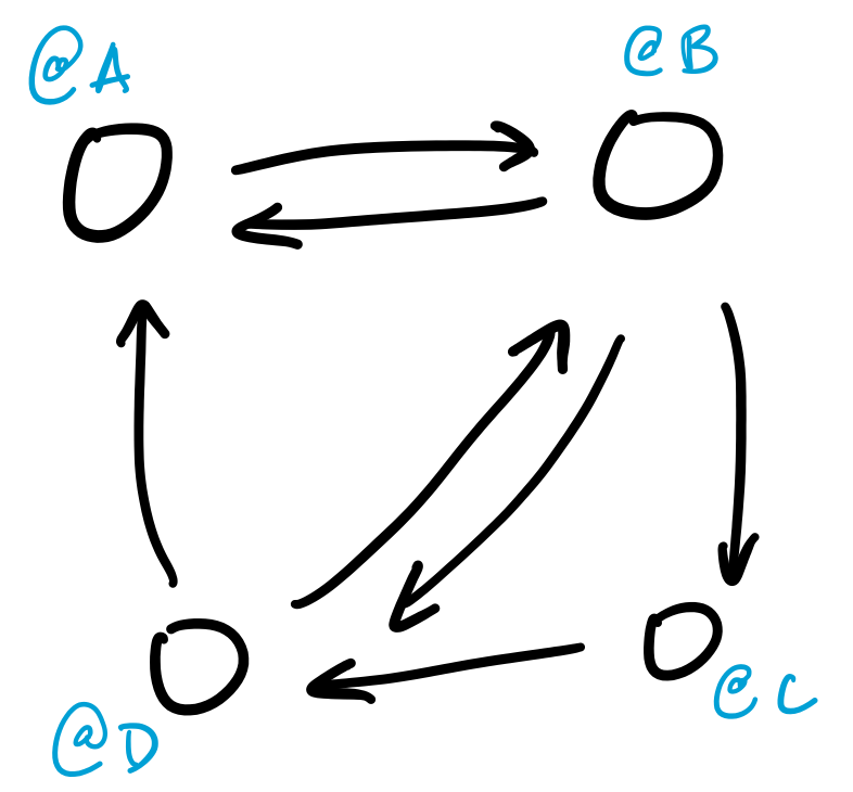
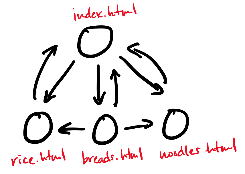
The web is a graph, where the vertices are webpages and the edges are links from one page to another. This model of the web is what informs many web search algorithms, like Google's PageRank, which measures the importance of a webpage based on how many incoming and outgoing links it has.
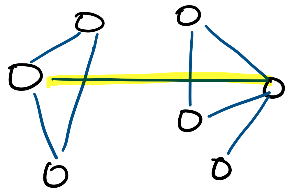
The Internet itself is a graph, where the vertices are the physical computers and the edges are the physical connections between them. Many computer networks can be viewed in this way. A common question that one can ask from this perspective is about minimum cuts. This is the question of what the cheapest way to disconnect the graph is, and therefore sever the network. This is a measure of the robustness of a network.
Graphs also have lots of non-network applications in computer science.
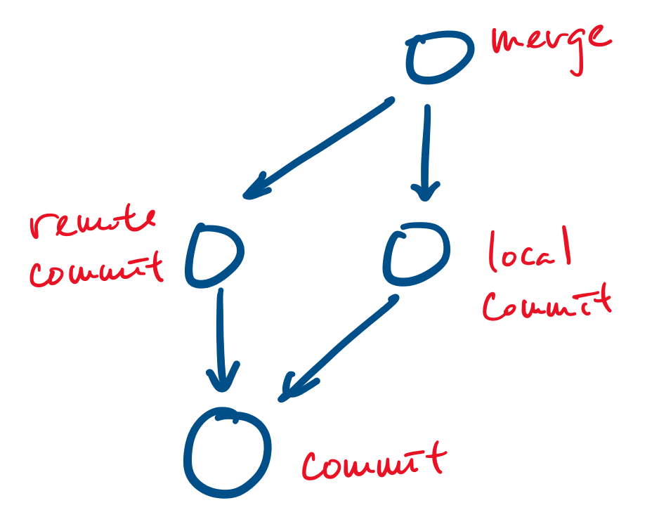
Your favourite revision control system, git, uses a graph based data model: all objects (such as files and commits) are represented as vertices and edges point from an object to an object that they depend on. For example, a commit is represented as a vertex and a merge can be represented as a vertex that points to the commits it merges.
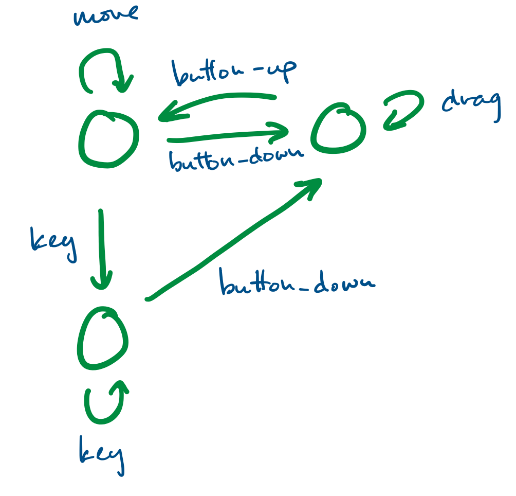
Finite state systems are often represented as graphs. These model the behaviour of complex systems, like software. For example, we can imagine that a program is in a "wait" state until a certain button has been pressed, at which point it moves to the appropriate state.
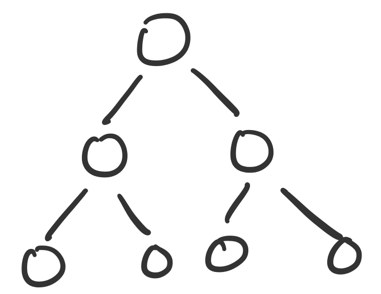
We've already made heavy use of a specific kind of graph: the binary tree. Trees, in general, are a class of graphs, specifically those that do not contain any cycles.
Graphs also model many real-world phenomena.
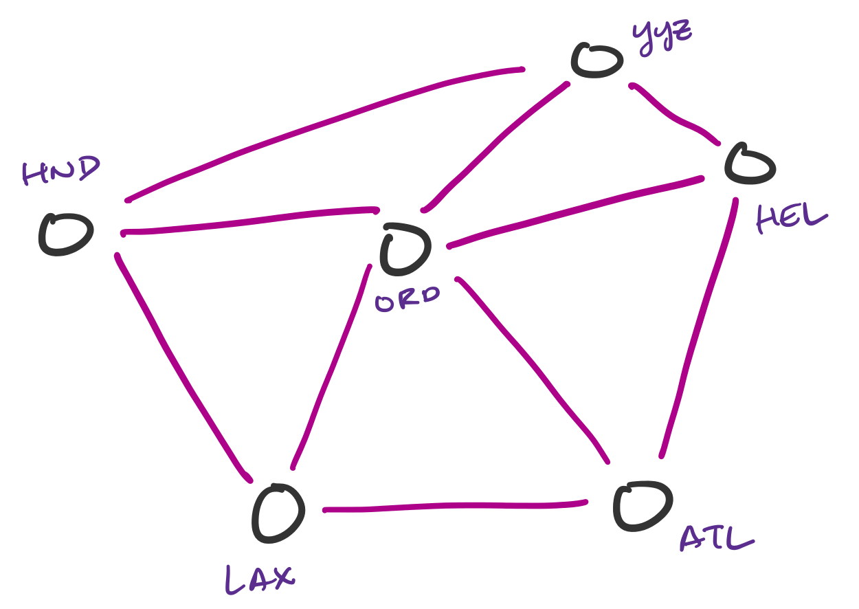
Transportation networks are commonly represented as graphs. These are not necessarily physical traffic networks, but more conceptual ones, like a flight network or a public transit network. One can then ask questions about the lowest-cost path from one node in the network to another.
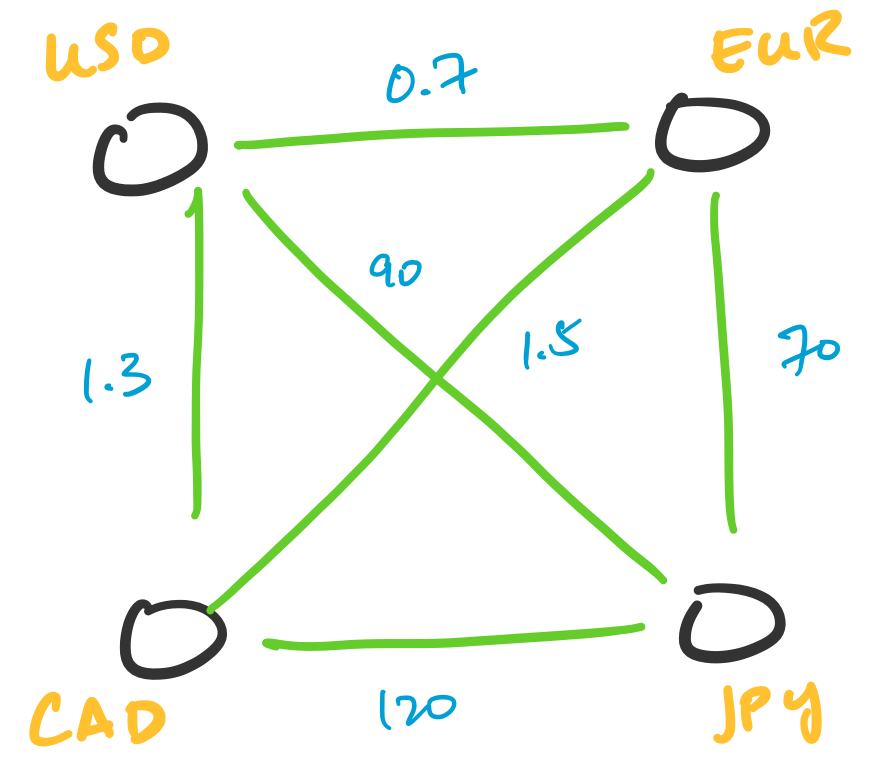
Transactions can be represented as graphs. One particularly interesting application of this is in currency arbitrage. In this setting, we represent currencies as vertices and assign weights to the edges corresponding to the exchange rate between two currencies. What makes this interesting is the fact that exchange rates can be totally independent of each other, which leads to opportunities for arbitrage. This involves indentifying cycles of a particular weight.
Many tasks can be reformulated as graphs. For instance, resource allocation is something that doesn't look like a graph problem, but can be turned into one. Suppose a university is trying to enroll students into classes in an upcoming quarter and students submit preferences for classes they would like to take. This can be modeled using a graph, and a possible assignment is a choice of a subset of edges.

You'll be familiar with the concept of graphs if you've taken courses in the introductory CS sequence. There, you are introduced to graphs as a data structure. Here, we'll be considering graphs as a mathematical object. As we've been seeing, this is actually not so different, except that we don't really have any "implementation details" to think about.
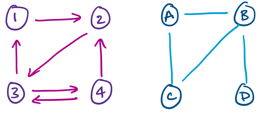
A graph $G = (V,E)$ is a pair with a non-empty set of vertices $V$ together with a set of edges $E$. An edge $e \in E$ is an unordered pair $(u,v)$ of vertices $u,v \in V$.
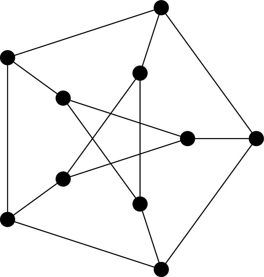
This graph is called the Petersen graph. The Petersen graph is a particularly interesting graph, not just because it looks neat, but because it happens to be a common counterexample for many results in graph theory.
From the definition, we immediately get that the edge set $E$ is a relation on $V \times V$. Furthermore, for undirected graphs, the edge relationship is always symmetric: $(u,v) \in E \rightarrow (v,u) \in E$. However, we don't treat these two pairs as different edges—they are considered one and the same.
One can define graphs more generally and then restrict consideration to our particular definition of graphs, which would usually be then called simple graphs. Instead, what we do is start with the most basic version of a graph, from which we can augment our definition with the more fancy features if necessary (it will not be necessary in this course).
For example, the above examples indicate that we can have a version of graphs in which edges have a direction, or where the edge relation is not enforced to be symmetric. These are directed graphs.
More general definitions of graphs also allow for things like multiple edges between vertices or loops.
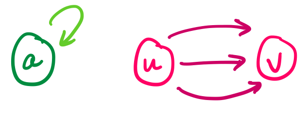
Other enhancements may include equipping edges with weights or even generalizing edges to hyperedges that relate more than two vertices.