We can think of some of the sample spaces we've seen already as describing independent events. For example, conisder the sample space of $\{H,T\}^n$. We can define the events $H_1$ to be the first coin flip was heads and $H_n$ to be the $n$th (or final) coin flip was heads and see that they are independent. Why? Intutiively, the first and last coin flips should have nothing to do with each other. If we're flipping a fair coin, the probability of these two events should be $\frac 1 2$. Independence tells us the probability of these two events occurring at the same time is exactly $\frac 1 4$.
Let's lay this out carefully. Since these are strings of length $n$, we can see that $H_1 = \{Hx \mid x \in \{H,T\}^n\}$ and $H_n = \{xH \mid x \in \{H,T\}^n\}$. We see that the probability of both events are $\frac 1 2$: $H_1$ consists of all strings of length $2^{n-1}$ prepended with $H$, which is half of all strings of length $2^n$ (the other half are the same strings prefixed with $T$). The same argument works for $H_n$.
Then what is $H_1 \cap H_n$? It is the set of strings $H \{H,T\}^{n-2} H$. This is exactly $\frac 1 4$ of the strings of length $n$, since to get the other $\frac 3 4$, we need to vary the $H$s at either end with $T$s.
It's worth pointing out here the difference between independence and disjointedness. The key lies in correctly interpreting the definition for disjointedness, which is that $\Pr(A \cap B) = 0$. If we go back to the definition, this says that $|A \cap B| = 0$. In other words, events $A$ and $B$ cannot and do not ever occur at the same time. On the other hand, independence tells us that $A$ and $B$ can occur at the same time, but they do not have any effect on each other. So in this sense, if $A$ and $B$ are disjoint, they are actually very dependent on each other.
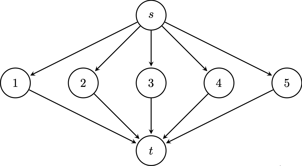
Consider the following directed graph. We want to get from the source $s$ to the destination $t$. However, each edge works independently with probability $p$. What is the probability that we can get from the source to the destination?
First, we note that there are only five paths, since this is a directed graph, and each path has two edges. Suppose $P_i$ is the event where there's a working path through vertex $i$. This gives us that $\Pr(P_i) = p^2$ for each $i$. Then if $P_{\text{exists}}$ is the event where there's at least one path from $s$ to $t$, then we put these together: \[\Pr(P_{\text{exists}}) = \Pr(P_1 \cup \cdots \cup P_5) = \Pr(P_1) + \cdots + \Pr(P_5) = 5p^2.\] Is this correct? Notice that if $p$ is large enough, say $p = \frac 3 4$, we end up with a probability over 1, which can't be true.
The bad assumption we made here was that we can just add the probabilities of the union—but we can only do that when the events are disjoint. But it can't be the case that our events are disjoint if the edge probabilities, and therefore, the path probabilties, are independent.
Let's be more careful. What's our sample space? One way to think about it is as a sequence, where we have $e_{1, \mathrm{in}} e_{1, \mathrm{out}} \cdots e_{5, \mathrm{in}} e_{5, \mathrm{out}}$ with each edge determined independently with probability $p$. Now, it's clear that $P_i$ and $P_j$ aren't disjoint—that is, they're not mutually exclusive.
So here's a trick/observation we can make: if what we want is the probability that there exists a path, this is the same as saying not all of the paths fail. In other words, \[\exists x P(x) \leftrightarrow \neg \neg \exists x P(x) \leftrightarrow \neg \forall x \neg P(x).\]
So we can express $P_1 \cup \cdots P_5$ as $\overline{\overline {P_1} \cap \cdots \cap \overline {P_5}}$ via De Morgan's laws. Now, these are still independent events but now we have an intersection. So this gives us \begin{align*} \Pr(P_{\text{exists}}) &= \Pr(P_1 \cup \cdots P_5) \\ &= 1 - \Pr(\overline {P_1} \cap \cdots {P_5}) \\\ &= 1 - \Pr(\overline {P_1}) \cdots \Pr(\overline {P_5}) \\ &= 1 - (1-p^2)^5, \end{align*} recalling that $\Pr(\overline{P_i}) = 1 - \Pr(P_i) = 1-p^2$. Another way to think about this is to observe that for each path, we consider the configurations of the two edges:
| Incoming edge works | Outgoing edge works | Probability |
|---|---|---|
| Yes | Yes | $p^2$ |
| Yes | No | $p(1-p)$ |
| No | Yes | $(1-p)p$ |
| No | No | $(1-p)^2$ |
Then \[p(1-p) + (1-p)p + (1-p)^2 = 2p-2p^2+1-2p+p^2 = 1-p^2, \] as expected.
An implicit assumption we've made here is that the path events are all mutually independent. This turns out to be a trickier definition than you might think.
Events $A_1, A_2, \dots, A_k$ are pairwise independent if for all $i \neq j$, $A_i$ and $A_j$ are independent. The events are mutually independent if for every $I \subseteq \{1, \dots, k\}$, $$\Pr \left( \bigcap_{i \in I} A_i \right) = \prod_{i \in I} \Pr(A_i).$$
The condition for mutual independence is quite strong. What it says is that for every subset of events, the probability of their intersection must be the product of their probabilities. If you have $k$ events, that's $\sum\limits_{j=2}^k \binom k j = 2^k-(k+1)$ different products to check.
This definition suggests that there can be events $A_1, A_2, \dots, A_k$ which are pairwise independent, but not mutually independent.
Consider flipping three fair coins and define the following events:
The sample space for these events is $\{H,T\}^3$. We can list the outcomes in each event:
Then we have that $\Pr(E_{12}) = \Pr(E_{13}) = \Pr(E_{23}) = \frac 4 8 = \frac 1 2$. Now, consider \[\Pr(E_{12} \cap E_{13}) = \Pr(\{HHH,TTT\}) = \frac 2 8 = \frac 1 4 = \frac 1 2 \cdot \frac 1 2 = \Pr(E_{12}) \cdot \Pr(E_{13}).\] So $E_{12}$ and $E_{13}$ are independent. And in fact $E_{13} \cap E_{23}$ and $E_{12} \cap E_{23}$ are both also $\{HHH,TTT\}$, so they are also independent. But then \[\Pr(E_{12} \cap E_{13} \cap E_{23}) = \Pr(\{HHH,TTT\}) = \frac 1 4 \neq \frac 1 8 = \Pr(E_{12}) \cdot \Pr(E_{13}) \cdot \Pr(E_{23}),\] so the three events are not mutually independent.
Generally, we would like to deal with mutually independent events, particularly if we have sequences of such events, like coin flips or dice rolls.
So far, we have been discussing and defining events but we can only ever talk about events occurring or not. But what if we wanted to say something about the events? That is, we'd like to discuss some value based on events. This is the idea behind random variables.
A random variable is a function $X : \Omega \to \mathbb R$ where $\Omega$ is the sample space of a probability space.
Suppose we roll two dice. Then $\Omega = \{1, \dots, 6\}^2$. We can define the random variable $X$ to be the sum of the two rolls. That is, $X(i,j) = i+j$.
Now, you may have noticed from our discussion that random variables are not random and are not variables (a random variable is a function, as we can see from the definition above, which is deterministic). This naming is due to Francesco Cantelli, from the early 1900s.
We notice that while random variables are functions, the standard usage is to really write them as though they're variables. So you will see things written like $X = r$ when what is really meant is $X(\omega) = r$ for some $\omega \in \Omega$.
Note that since we're dealing with finite and discrete probability spaces, a lot of the time, we'll be mapping outcomes to discrete codomains like $\mathbb N$ or $\{0,1\}$. And while the standard definition of a random variable is for $\mathbb R$, this can be extended to more exotic co-domains than just $\mathbb R$.
Having set up this mechanism, we can define the probability of a particular outcome of a random variable.
If $X$ is a random variable, the probability that $X = r$, for some $r \in \mathbb R$ is defined by $\Pr(X = r) = \Pr(\{\omega \in \Omega \mid X(\omega) = r\})$.
This is pretty straightforward: the probability that a random variable $X$ takes on a value $r$ is just the probability of the outcomes that $X$ assigns to $r$.
From this, the simplest example of a random variable is the random variable that just describes whether an event occurs or not. These are called indicator random variables or just indicator variables.
For an event $A$, the indicator variable $I_A$ is a function $I_A : \Omega \to \{0,1\}$ which is defined by \[I_A(\omega) = \begin{cases} 1 & \text{if $\omega \in A$}, \\ 0 & \text{if $\omega \not \in A$}. \end{cases} \] These are also called Bernoulli random variables, framed as the outcome of a "Bernoulli trial" so that if the indicator $X$ takes on $X = 1$, it's considered a "success" and $X = 0$ is a "failure".
Bernoulli random variables are named so, after Jacob Bernoulli who is also sometimes referred to as James Bernoulli in the late 1600s. There are lots of other mathematicians in the Bernoulli family but the lion's share of mathematical results named after Bernoulli are really named after this particular Bernoulli.
Suppose we flip a coin three times. Let $X(\omega)$ be the random variable that equals the number of heads that appear when $\omega$ is the outcome. So we have \begin{align*} X(HHH) &= 3, \\ X(HHT) = X(HTH) = X(THH) &= 2, \\ X(TTH) = X(THT) = X(HHT) &= 1, \\ X(TTT) &= 0. \end{align*} Now, suppose that the coin is fair. Since we assume that each of the coin flips is mutually independent, this gives us a probability of $\frac 1 2 \frac 1 2 \frac 1 2 = \frac 1 8$ for any one of the above outcomes. Now, let's consider $\Pr(X = k)$:
| $k$ | $\{\omega \in \Omega \mid X(\omega) = k\}$ | $\Pr(X = k)$ |
|---|---|---|
| 3 | $\{HHH\}$ | $\frac 1 8$ |
| 2 | $\{HHT,HTH,THH\}$ | $\frac 3 8$ |
| 1 | $\{TTH,THT,HTT\}$ | $\frac 3 8$ |
| 0 | $\{TTT\}$ | $\frac 1 8$ |
At this point, this doesn't seem particularly useful over what we've already been doing, so let's consider a more complicated example.
Consider the sample space of graphs with $n$ vertices. It's not immediately obvious how we should assign probabilities to these graphs. One way to do this, due to Erdős and Rényi, is to then consider those graphs with $m$ edges as the sample space and have them uniformly distributed. (In this case, what is the probability of getting a single graph?)
Another model is to consider all the graphs of $n$ vertices but instead of trying to assign a distribution to the graphs directly, we assign probabilities to the presence of edges, like the example we did above with the directed graph. We consider each edge independently and include it in our graph with probability $p$. Unlike before, this doesn't really give us a clear picture of what the probability of a particular graph is. Instead, we need to consider such questions using random variables.
We can consider the presence of an edge an indicator—that is, we define a random variable $E_{u,v}$ to be 1 if the edge is present in the graph and 0 if not. Formally, \[E_{u,v} = \begin{cases} 1 & \text{if $(u,v) \in E$}, \\ 0 & \text{if $(u,v) \not \in E$}. \end{cases}\] Then we can define another random variable, say $E_{\mathrm{total}}$ to be the number edges in our random graph, defined by \[E_{\mathrm{total}} = \sum_{u,v \in V} E_{u,v}.\] With this, we can ask something like what the probability of a graph having $m$ edges is. In other words, what is $\Pr(E_{\mathrm{total}} = m)$?
Since these are independent, we can consider each $E_{u,v}$ independently. Then since there are $\binom n 2$ such random variables, we put the probabilities together to find that any particular graph with $m$ edges occurs with probability $p^m (1-p)^{\binom n 2 - m}$. That is, there are exactly $m$ edges included (with probability $p$) and the rest are excluded with probability $1-p$, and there are exactly $\binom n 2 - m$ of these.
Finally, noting that there are $\binom{\binom n 2} m$ ways to choose $m$ edges from $n$ vertices, we have that the probability that we get some graph with $m$ edges is \[\binom{\binom n 2}m p^m (1-p)^{\binom n 2 - m}.\]